WannierBerri advanced tutorial - Fermi surface and Fermi sea calculation of the Berry curvature dipole
author: Jae-Mo Lihm (jaemo.lihm@gmail.com)
The Berry curvature dipole (BCD) is the dipole of the Berry curvature in the reciprocal space. BCD has attracted considerable attention, partially because it contributes to the nonlinear Hall effect.
In WannierBerri, there are two ways to compute this quantity: the Fermi surface integral and the Fermi sea integral:
Formally, one can show that the two methods give identical results using partial integration:
The integral is zero because the Brillouin zone has no boundary.
However, in practice, there are numerical differences between the two methods. In this tutorial, we compare the Fermi sea and Fermi surface integral methods for the BCD using the chiral tight-binding model and the ab-initio tight-binding model of ferroelectric GeTe.
[1]:
# Preliminary (Do only once)
%load_ext autoreload
%autoreload 2

# Set environment variables - not mandatory but recommended
import os
os.environ['OPENBLAS_NUM_THREADS'] = '1'
os.environ['MKL_NUM_THREADS'] = '1'

import numpy as np
import matplotlib.pyplot as plt
import wannierberri as wberri
from wannierberri import calculators as calc

import ray
ray.init(num_cpus=24)
/home/stepan/github/WannierBerri-tutorial/.conda/lib/python3.12/site-packages/tqdm/auto.py:21: TqdmWarning: IProgress not found. Please update jupyter and ipywidgets. See https://ipywidgets.readthedocs.io/en/stable/user_install.html
  from .autonotebook import tqdm as notebook_tqdm
2026-03-30 23:37:58,622 INFO util.py:154 -- Missing packages: ['ipywidgets']. Run `pip install -U ipywidgets`, then restart the notebook server for rich notebook output.
2026-03-30 23:38:00,354 INFO worker.py:1918 -- Started a local Ray instance. View the dashboard at http://127.0.0.1:8266
[1]:
| Python version: | 3.12.12 |
| Ray version: | 2.48.0 |
| Dashboard: | http://127.0.0.1:8266 |
Model 1: Chiral tight-binding model
Model, band structure
The model is taken from T. Yoda et al, “Orbital Edelstein Effect as a Condensed-Matter Analog of Solenoids”, Nano Lett. 18, 2, 916–920 (2018) https://arxiv.org/abs/1706.07702
The system is a honeycomb lattice with two orbitals per unit cell with an AA stacking (i.e. an AA stacked 2d hexagonal boron nitride). The original model contains in-plance nearest-neighbor hopping (hop1), vertical hopping (hopz_vert), and chiral inter-layer hopping (hopz_left and hopz_right). Here, we additionally add onsite energy difference (delta) and in-plane next-nearest-neighbor hopping (hop2 and phi). Nonzero phi breaks the time-reversal symmetry.
When we set phi=0, the model has time-reversal symmetry and C3z symmetry. In total, there are 6 symmetry operations.
[2]:
import wannierberri.models

# Initiate a tight-binding model (wannierberri.models.Chiral uses PythTB)
model_Chiral_left = wannierberri.models.Chiral(delta=2., hop1=1., hop2=0.3, phi=0, hopz_left=0.2, hopz_right=0.0, hopz_vert=0)

# Initialize WannierBerri system object
system = wberri.System_R.from_pythtb(model_Chiral_left)

print("=" * 40)

# Set symmetry from the generators.
system.set_pointgroup(symmetry_gen=["TimeReversal", "C3z"])
print("Number of symmetry operations: ", system.pointgroup.size)
Reading the system from PythTB model. Needed data: {'Ham'}
number of wannier functions: 2
shape of Ham_R = (21, 2, 2)
Real-space lattice:
 [[1.        0.        0.       ]
 [0.5       0.8660254 0.       ]
 [0.        0.        1.       ]]
Number of wannier functions: 2
Number of R points: 21
Recommended size of FFT grid [3 3 3]
Reading the system from PythTB finished successfully
========================================
Number of symmetry operations:  6
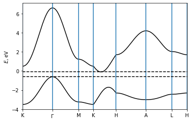
Now, we plot the band structure along a k-point path that passes the high-symmetry k points. We use the plot_path_fat method to plot the band structure.
The energy can be accessed via path_result.get_data("Energy", iband). The valence band maximum is at the Gamma point, while the conduction band minimum on the K-H line.

Figure taken from T. Yoda et al, Nano Lett. 18, 2, 916–920 (2018).
[3]:
path = wberri.Path.from_nodes(
    system,
    nodes=[
        [2/3, 1/3, 0.],  #  K
        [0.,  0.,  0.],  #  Gamma
        [1/2, 0.,  0.],  #  M
        [2/3, 1/3, 0.],  #  K
        [2/3, 1/3, 0.5],  #  H
        [0.,  0.,  0.5],  #  A
        [1/2, 0.,  0.5],  #  L
        [2/3, 1/3, 0.5],  #  H
    ],
    labels=["K","$\Gamma$","M","K", "H", "A", "L", "H"],
    length=50
)


bands = wberri.evaluate_k_path(
    system=system,
    path=path,
)
Starting run()
Using the follwing calculators :
############################################################

 'tabulate'  :  <wannierberri.calculators.tabulate.TabulatorAll object at 0x7d9c214814c0>  :
    TabulatorAll - a pack of all k-resolved calculators (Tabulators)

 Includes the following tabulators :
--------------------------------------------------
 "Energy" : <wannierberri.calculators.tabulate.Energy object at 0x7d9bc85ab200> : calculator not described

--------------------------------------------------

############################################################
Calculation along a path - checking calculators for compatibility
tabulate <wannierberri.calculators.tabulate.TabulatorAll object at 0x7d9c214814c0>
All calculators are compatible
Symmetrization switched off for Path
Grid is regular
The set of k points is a Path() with 184 points and labels {0: 'K', 33: '$\\Gamma$', 62: 'M', 79: 'K', 104: 'H', 137: 'A', 166: 'L', 183: 'H'}
generating K_list
Done
Done, sum of weights:184.0

############################################################
Iteration 0 out of 0
processing 184 K points : using  24 processes.
# K-points calculated  Wall time (sec)  Est. remaining (sec)   Est. total (sec)
/home/stepan/github/wannier-berri/wannierberri/grid/path.py:272: UserWarning: symmetry is not used for a tabulation along path
  warnings.warn("symmetry is not used for a tabulation along path")
time for processing    184 K-points on  24 processes:     0.8007 ; per K-point          0.0044 ; proc-sec per K-point          0.1044
time1 =  4.76837158203125e-07
Totally processed 184 K-points
run() finished
[4]:
e_vbm = np.amax(bands.get_data("Energy", 0))
e_cbm = np.amin(bands.get_data("Energy", 1))
print(f"Valence band maximum   : {e_vbm:6.3f}")
print(f"Conduction band minimum: {e_cbm:6.3f}")

print("VBM k point: ", bands.kpoints[np.argmax(bands.get_data("Energy", 0))])
print("CBM k point: ", bands.kpoints[np.argmin(bands.get_data("Energy", 1))])

fig = bands.plot_path_fat(path, close_fig=False, show_fig=False)

ax = fig.get_axes()[0]
ax.axhline(e_vbm, c="k", ls="--")
ax.axhline(e_cbm, c="k", ls="--")
plt.show(fig)
Valence band maximum   : -0.606
Conduction band minimum: -0.099
VBM k point:  [0. 0. 0.]
CBM k point:  [0.66666667 0.33333333 0.16      ]
Berry curvature dipole
[5]:
from wannierberri.smoother import FermiDiracSmoother

efermi = np.linspace(-2.0, 1.0, 101, True)
# efermi = np.linspace(e_vbm - 0.5, e_cbm + 0.5, 301, True)

kwargs = dict(
    Efermi=efermi,
    kwargs_formula={"external_terms": False},
    smoother=FermiDiracSmoother(efermi, T_Kelvin=1200, maxdE=8)
)

calculators = {
    'berry_dipole_fermi_sea': calc.static.BerryDipole_FermiSea(**kwargs),
    'berry_dipole_fermi_surface': calc.static.BerryDipole_FermiSurf(**kwargs),
    'dos': calc.static.DOS(Efermi=efermi,),
}
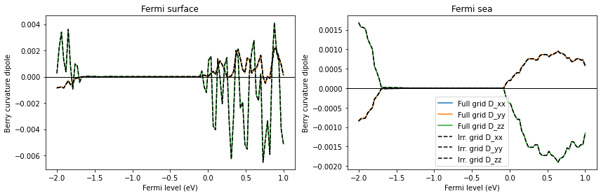
Compare calculations using the full k-point grid and the irreducible grid. This can be done using the use_irred_kpt argument of wberri.run.
You can find the following two lines in the output: K_list contains 1000 Irreducible points(100.0%) out of initial 10x10x10=1000 grid K_list contains 172 Irreducible points(17.2%) out of initial 10x10x10=1000 grid
These lines show that using symmetry can speed up calculation by 1000 / 172 ~ 6 times. This speedup corresponds to the 6 symmetry operations. Check that the BCD calculated from the two grids are identical.
[6]:
grid = wberri.Grid(system, NK=20, NKFFT=2)
print("=" * 40)
print("Calculation using the full k-point grid")
result_full_grid = wberri.run(
    system,
    grid=grid,
    calculators=calculators,
    print_Kpoints = False,
    use_irred_kpt = False,
)

print("=" * 40)
print("Calculation using the irreducible k-point grid")
result_irr_grid = wberri.run(
    system,
    grid=grid,
    calculators=calculators,
    print_Kpoints = False,
    use_irred_kpt = True,
)
========================================
Calculation using the full k-point grid
Starting run()
Using the follwing calculators :
############################################################

 'berry_dipole_fermi_sea'  :  <wannierberri.calculators.static.BerryDipole_FermiSea object at 0x7d9bc82574d0>  : Berry curvature dipole (dimensionless)

        | With Fermi sea integral. Eq(29) in `Ref <https://www.nature.com/articles/s41524-021-00498-5>`__
        | Output: :math:`D_{\beta\delta} = \int [dk] \partial_\beta \Omega_\delta f`
 'berry_dipole_fermi_surface'  :  <wannierberri.calculators.static.BerryDipole_FermiSurf object at 0x7d9bc8256900>  : Berry curvature dipole (dimensionless)

        | With Fermi surface integral. Eq(8) in `Ref <https://journals.aps.org/prl/abstract/10.1103/PhysRevLett.115.216806>`__
        | Output: :math:`D_{\beta\delta} = -\int [dk] v_\beta \Omega_\delta f'`
 'dos'  :  <wannierberri.calculators.static.DOS object at 0x7d9bc8257050>  : Density of states
############################################################
Calculation on  grid - checking calculators for compatibility
berry_dipole_fermi_sea <wannierberri.calculators.static.BerryDipole_FermiSea object at 0x7d9bc82574d0>
berry_dipole_fermi_surface <wannierberri.calculators.static.BerryDipole_FermiSurf object at 0x7d9bc8256900>
dos <wannierberri.calculators.static.DOS object at 0x7d9bc8257050>
All calculators are compatible
Grid is regular
The set of k points is a Grid() with NKdiv=[10 10 10], NKFFT=[2 2 2], NKtot=[20 20 20]
generating K_list
Done in 0.002751588821411133 s
K_list contains 1000 Irreducible points(100.0%) out of initial 10x10x10=1000 grid
Done, sum of weights:1.0000000000000007

############################################################
Iteration 0 out of 0
processing 1000 K points : using  24 processes.
# K-points calculated  Wall time (sec)  Est. remaining (sec)   Est. total (sec)
time for processing   1000 K-points on  24 processes:     3.8073 ; per K-point          0.0038 ; proc-sec per K-point          0.0914
time1 =  2.384185791015625e-07
Totally processed 1000 K-points
run() finished
========================================
Calculation using the irreducible k-point grid
Starting run()
Using the follwing calculators :
############################################################

 'berry_dipole_fermi_sea'  :  <wannierberri.calculators.static.BerryDipole_FermiSea object at 0x7d9bc82574d0>  : Berry curvature dipole (dimensionless)

        | With Fermi sea integral. Eq(29) in `Ref <https://www.nature.com/articles/s41524-021-00498-5>`__
        | Output: :math:`D_{\beta\delta} = \int [dk] \partial_\beta \Omega_\delta f`
 'berry_dipole_fermi_surface'  :  <wannierberri.calculators.static.BerryDipole_FermiSurf object at 0x7d9bc8256900>  : Berry curvature dipole (dimensionless)

        | With Fermi surface integral. Eq(8) in `Ref <https://journals.aps.org/prl/abstract/10.1103/PhysRevLett.115.216806>`__
        | Output: :math:`D_{\beta\delta} = -\int [dk] v_\beta \Omega_\delta f'`
 'dos'  :  <wannierberri.calculators.static.DOS object at 0x7d9bc8257050>  : Density of states
############################################################
Calculation on  grid - checking calculators for compatibility
berry_dipole_fermi_sea <wannierberri.calculators.static.BerryDipole_FermiSea object at 0x7d9bc82574d0>
berry_dipole_fermi_surface <wannierberri.calculators.static.BerryDipole_FermiSurf object at 0x7d9bc8256900>
dos <wannierberri.calculators.static.DOS object at 0x7d9bc8257050>
All calculators are compatible
Grid is regular
The set of k points is a Grid() with NKdiv=[10 10 10], NKFFT=[2 2 2], NKtot=[20 20 20]
generating K_list
Done in 0.0023720264434814453 s
excluding symmetry-equivalent K-points from initial grid
Done in 0.01342010498046875 s
K_list contains 172 Irreducible points(17.2%) out of initial 10x10x10=1000 grid
Done, sum of weights:1.0000000000000007

############################################################
Iteration 0 out of 0
processing 172 K points : using  24 processes.
# K-points calculated  Wall time (sec)  Est. remaining (sec)   Est. total (sec)
time for processing    172 K-points on  24 processes:     0.4138 ; per K-point          0.0024 ; proc-sec per K-point          0.0577
time1 =  4.76837158203125e-07
Totally processed 172 K-points
run() finished
[7]:
dir_string = ["D_xx", "D_yy", "D_zz"]

fig, axes = plt.subplots(1, 2, figsize=(12, 4))
for label, res in zip(["Full grid", "Irr. grid"], [result_full_grid, result_irr_grid]):
    data_fsurf = res.results['berry_dipole_fermi_surface'].data
    data_fsea = res.results['berry_dipole_fermi_sea'].data
    for i in range(3):
        if label == "Full grid":
            fmt = f"C{i}-"
        else:
            fmt = "k--"
        axes[0].plot(efermi, data_fsurf[:, i, i], fmt, label=label + " " + dir_string[i])
        axes[1].plot(efermi, data_fsea[:, i, i], fmt, label=label + " " + dir_string[i])

axes[0].set_title("Fermi surface")
axes[1].set_title("Fermi sea")

for ax in axes:
    ax.axhline(0, c="k", lw=1)
    ax.set_xlabel("Fermi level (eV)")
    ax.set_ylabel("Berry curvature dipole")

axes[1].legend()
plt.tight_layout()
plt.show()
From now on, we use the irreducible k-point grid, which is the default in wberri.run.
[8]:
grid = wberri.Grid(system, NK=20, NKFFT=2)
result = wberri.run(
    system,
    grid=grid,
    calculators=calculators,
    print_Kpoints = False,
)
Starting run()
Using the follwing calculators :
############################################################

 'berry_dipole_fermi_sea'  :  <wannierberri.calculators.static.BerryDipole_FermiSea object at 0x7d9bc82574d0>  : Berry curvature dipole (dimensionless)

        | With Fermi sea integral. Eq(29) in `Ref <https://www.nature.com/articles/s41524-021-00498-5>`__
        | Output: :math:`D_{\beta\delta} = \int [dk] \partial_\beta \Omega_\delta f`
 'berry_dipole_fermi_surface'  :  <wannierberri.calculators.static.BerryDipole_FermiSurf object at 0x7d9bc8256900>  : Berry curvature dipole (dimensionless)

        | With Fermi surface integral. Eq(8) in `Ref <https://journals.aps.org/prl/abstract/10.1103/PhysRevLett.115.216806>`__
        | Output: :math:`D_{\beta\delta} = -\int [dk] v_\beta \Omega_\delta f'`
 'dos'  :  <wannierberri.calculators.static.DOS object at 0x7d9bc8257050>  : Density of states
############################################################
Calculation on  grid - checking calculators for compatibility
berry_dipole_fermi_sea <wannierberri.calculators.static.BerryDipole_FermiSea object at 0x7d9bc82574d0>
berry_dipole_fermi_surface <wannierberri.calculators.static.BerryDipole_FermiSurf object at 0x7d9bc8256900>
dos <wannierberri.calculators.static.DOS object at 0x7d9bc8257050>
All calculators are compatible
Grid is regular
The set of k points is a Grid() with NKdiv=[10 10 10], NKFFT=[2 2 2], NKtot=[20 20 20]
generating K_list
Done in 0.0025815963745117188 s
excluding symmetry-equivalent K-points from initial grid
Done in 0.012717485427856445 s
K_list contains 172 Irreducible points(17.2%) out of initial 10x10x10=1000 grid
Done, sum of weights:1.0000000000000007

############################################################
Iteration 0 out of 0
processing 172 K points : using  24 processes.
# K-points calculated  Wall time (sec)  Est. remaining (sec)   Est. total (sec)
time for processing    172 K-points on  24 processes:     0.3898 ; per K-point          0.0023 ; proc-sec per K-point          0.0544
time1 =  2.384185791015625e-07
Totally processed 172 K-points
run() finished
[9]:
data_fsurf = result.results['berry_dipole_fermi_surface'].data
data_fsea = result.results['berry_dipole_fermi_sea'].data

print("Shape of data: ", data_fsurf.shape)

print("Maximum value for each components (Fermi surface): ")
print(np.linalg.norm(data_fsurf, axis=0))

print("Maximum value for each components (Fermi sea): ")
print(np.linalg.norm(data_fsea, axis=0))
Shape of data:  (101, 3, 3)
Maximum value for each components (Fermi surface):
[[6.62623214e-03 3.93194983e-04 5.47673978e-18]
 [3.93194983e-04 6.62623214e-03 1.09199268e-18]
 [8.49488438e-19 1.87590102e-19 1.99418701e-02]]
Maximum value for each components (Fermi sea):
[[4.66910328e-03 2.46816267e-04 1.44728124e-17]
 [2.46816267e-04 4.66910328e-03 1.51001947e-18]
 [5.49317581e-19 2.66514580e-19 9.33820656e-03]]
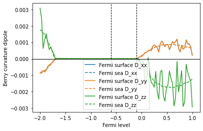
[10]:
dir_string = ["D_xx", "D_yy", "D_zz"]
for i in range(3):
    plt.plot(efermi, data_fsurf[:, i, i], c=f"C{i}", label="Fermi surface " + dir_string[i])
    plt.plot(efermi, data_fsea[:, i, i], c=f"C{i}", label="Fermi sea " + dir_string[i], ls="--")

# plt.plot(efermi, result.results['dos'].data, "k-")

plt.axhline(0, c="k", lw=1)
plt.xlabel("Fermi level")
plt.ylabel("Berry curvature dipole")
plt.axvline(e_vbm, c="k", lw=1, ls="--")
plt.axvline(e_cbm, c="k", lw=1, ls="--")
plt.legend()
plt.show()
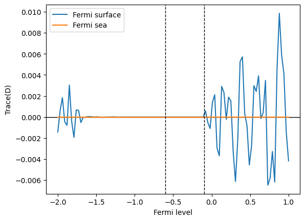
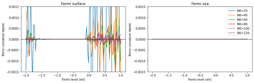
The trace of the BCD tensor should be zero due to a topological reason (see footnote 2 of S.Tsirkin et al, PRB 97, 035158 (2018) for details).
The Fermi sea formula for the BCD tensor is explicitly traceless at every k point: this fact can be proven from the definition of the Fermi sea formula using
In contrast, tracelessness is not explicit in the Fermi surface formula. The trace of the BCD tensor becomes zero only after summing over the full Brillouin zone due to the cancellation of contributions from all the k points.
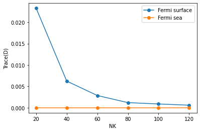
Therefore, in numerical calculations using a finite number of k points, only the Fermi sea formula, not the Fermi surface formula, gives a zero trace. The trace will converge to 0 in the Fermi surface case as one makes the k-point grid denser.
[11]:
data_fsurf_trace = np.trace(data_fsurf, axis1=1, axis2=2)
data_fsea_trace = np.trace(data_fsea, axis1=1, axis2=2)

plt.plot(efermi, data_fsurf_trace, label="Fermi surface")
plt.plot(efermi, data_fsea_trace, label="Fermi sea")

plt.axhline(0, c="k", lw=1, zorder=1)
plt.xlabel("Fermi level")
plt.ylabel("Trace(D)")
plt.axvline(e_vbm, c="k", lw=1, ls="--")
plt.axvline(e_cbm, c="k", lw=1, ls="--")
plt.legend()
plt.show()
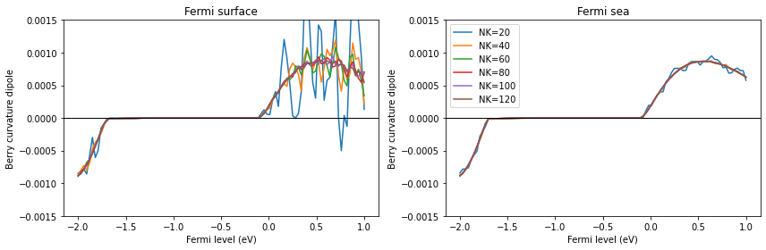
Try to calculate the Berry curvature dipole using the two methods for various grid sizes and see how they converge. Also, check that the trace of Berry curvature dipole indeed converges to 0 for both methods.
(NK=120 will be enough to see convergence.)
[12]:
data_fsurf_all = {}
data_fsea_all = {}
[13]:
for nk in [20, 40, 60, 80]:
    grid = wberri.Grid(system, NK=nk, NKFFT=10)
    result = wberri.run(
        system,
        grid=grid,
        calculators=calculators,
        print_Kpoints = False,
    )
    data_fsurf_all[nk] = result.results['berry_dipole_fermi_surface'].data
    data_fsea_all[nk] = result.results['berry_dipole_fermi_sea'].data
Starting run()
Using the follwing calculators :
############################################################

 'berry_dipole_fermi_sea'  :  <wannierberri.calculators.static.BerryDipole_FermiSea object at 0x7d9bc82574d0>  : Berry curvature dipole (dimensionless)

        | With Fermi sea integral. Eq(29) in `Ref <https://www.nature.com/articles/s41524-021-00498-5>`__
        | Output: :math:`D_{\beta\delta} = \int [dk] \partial_\beta \Omega_\delta f`
 'berry_dipole_fermi_surface'  :  <wannierberri.calculators.static.BerryDipole_FermiSurf object at 0x7d9bc8256900>  : Berry curvature dipole (dimensionless)

        | With Fermi surface integral. Eq(8) in `Ref <https://journals.aps.org/prl/abstract/10.1103/PhysRevLett.115.216806>`__
        | Output: :math:`D_{\beta\delta} = -\int [dk] v_\beta \Omega_\delta f'`
 'dos'  :  <wannierberri.calculators.static.DOS object at 0x7d9bc8257050>  : Density of states
############################################################
Calculation on  grid - checking calculators for compatibility
berry_dipole_fermi_sea <wannierberri.calculators.static.BerryDipole_FermiSea object at 0x7d9bc82574d0>
berry_dipole_fermi_surface <wannierberri.calculators.static.BerryDipole_FermiSurf object at 0x7d9bc8256900>
dos <wannierberri.calculators.static.DOS object at 0x7d9bc8257050>
All calculators are compatible
Grid is regular
The set of k points is a Grid() with NKdiv=[2 2 2], NKFFT=[10 10 10], NKtot=[20 20 20]
generating K_list
Done in 9.822845458984375e-05 s
excluding symmetry-equivalent K-points from initial grid
Done in 0.0005297660827636719 s
K_list contains 4 Irreducible points(50.0%) out of initial 2x2x2=8 grid
Done, sum of weights:1.0

############################################################
Iteration 0 out of 0
processing 4 K points : using  24 processes.
# K-points calculated  Wall time (sec)  Est. remaining (sec)   Est. total (sec)
time for processing      4 K-points on  24 processes:     0.4064 ; per K-point          0.1016 ; proc-sec per K-point          2.4383
time1 =  2.384185791015625e-07
Totally processed 4 K-points
run() finished
Starting run()
Using the follwing calculators :
############################################################

 'berry_dipole_fermi_sea'  :  <wannierberri.calculators.static.BerryDipole_FermiSea object at 0x7d9bc82574d0>  : Berry curvature dipole (dimensionless)

        | With Fermi sea integral. Eq(29) in `Ref <https://www.nature.com/articles/s41524-021-00498-5>`__
        | Output: :math:`D_{\beta\delta} = \int [dk] \partial_\beta \Omega_\delta f`
 'berry_dipole_fermi_surface'  :  <wannierberri.calculators.static.BerryDipole_FermiSurf object at 0x7d9bc8256900>  : Berry curvature dipole (dimensionless)

        | With Fermi surface integral. Eq(8) in `Ref <https://journals.aps.org/prl/abstract/10.1103/PhysRevLett.115.216806>`__
        | Output: :math:`D_{\beta\delta} = -\int [dk] v_\beta \Omega_\delta f'`
 'dos'  :  <wannierberri.calculators.static.DOS object at 0x7d9bc8257050>  : Density of states
############################################################
Calculation on  grid - checking calculators for compatibility
berry_dipole_fermi_sea <wannierberri.calculators.static.BerryDipole_FermiSea object at 0x7d9bc82574d0>
berry_dipole_fermi_surface <wannierberri.calculators.static.BerryDipole_FermiSurf object at 0x7d9bc8256900>
dos <wannierberri.calculators.static.DOS object at 0x7d9bc8257050>
All calculators are compatible
Grid is regular
The set of k points is a Grid() with NKdiv=[4 4 4], NKFFT=[10 10 10], NKtot=[40 40 40]
generating K_list
Done in 0.00022530555725097656 s
excluding symmetry-equivalent K-points from initial grid
Done in 0.0013856887817382812 s
K_list contains 14 Irreducible points(21.88%) out of initial 4x4x4=64 grid
Done, sum of weights:1.0

############################################################
Iteration 0 out of 0
processing 14 K points : using  24 processes.
# K-points calculated  Wall time (sec)  Est. remaining (sec)   Est. total (sec)
time for processing     14 K-points on  24 processes:     0.6109 ; per K-point          0.0436 ; proc-sec per K-point          1.0472
time1 =  2.384185791015625e-07
Totally processed 14 K-points
run() finished
Starting run()
Using the follwing calculators :
############################################################

 'berry_dipole_fermi_sea'  :  <wannierberri.calculators.static.BerryDipole_FermiSea object at 0x7d9bc82574d0>  : Berry curvature dipole (dimensionless)

        | With Fermi sea integral. Eq(29) in `Ref <https://www.nature.com/articles/s41524-021-00498-5>`__
        | Output: :math:`D_{\beta\delta} = \int [dk] \partial_\beta \Omega_\delta f`
 'berry_dipole_fermi_surface'  :  <wannierberri.calculators.static.BerryDipole_FermiSurf object at 0x7d9bc8256900>  : Berry curvature dipole (dimensionless)

        | With Fermi surface integral. Eq(8) in `Ref <https://journals.aps.org/prl/abstract/10.1103/PhysRevLett.115.216806>`__
        | Output: :math:`D_{\beta\delta} = -\int [dk] v_\beta \Omega_\delta f'`
 'dos'  :  <wannierberri.calculators.static.DOS object at 0x7d9bc8257050>  : Density of states
############################################################
Calculation on  grid - checking calculators for compatibility
berry_dipole_fermi_sea <wannierberri.calculators.static.BerryDipole_FermiSea object at 0x7d9bc82574d0>
berry_dipole_fermi_surface <wannierberri.calculators.static.BerryDipole_FermiSurf object at 0x7d9bc8256900>
dos <wannierberri.calculators.static.DOS object at 0x7d9bc8257050>
All calculators are compatible
Grid is regular
The set of k points is a Grid() with NKdiv=[6 6 6], NKFFT=[10 10 10], NKtot=[60 60 60]
generating K_list
Done in 0.0005817413330078125 s
excluding symmetry-equivalent K-points from initial grid
Done in 0.0038895606994628906 s
K_list contains 44 Irreducible points(20.37%) out of initial 6x6x6=216 grid
Done, sum of weights:1.0000000000000004

############################################################
Iteration 0 out of 0
processing 44 K points : using  24 processes.
# K-points calculated  Wall time (sec)  Est. remaining (sec)   Est. total (sec)
time for processing     44 K-points on  24 processes:     1.4703 ; per K-point          0.0334 ; proc-sec per K-point          0.8020
time1 =  4.76837158203125e-07
Totally processed 44 K-points
run() finished
Starting run()
Using the follwing calculators :
############################################################

 'berry_dipole_fermi_sea'  :  <wannierberri.calculators.static.BerryDipole_FermiSea object at 0x7d9bc82574d0>  : Berry curvature dipole (dimensionless)

        | With Fermi sea integral. Eq(29) in `Ref <https://www.nature.com/articles/s41524-021-00498-5>`__
        | Output: :math:`D_{\beta\delta} = \int [dk] \partial_\beta \Omega_\delta f`
 'berry_dipole_fermi_surface'  :  <wannierberri.calculators.static.BerryDipole_FermiSurf object at 0x7d9bc8256900>  : Berry curvature dipole (dimensionless)

        | With Fermi surface integral. Eq(8) in `Ref <https://journals.aps.org/prl/abstract/10.1103/PhysRevLett.115.216806>`__
        | Output: :math:`D_{\beta\delta} = -\int [dk] v_\beta \Omega_\delta f'`
 'dos'  :  <wannierberri.calculators.static.DOS object at 0x7d9bc8257050>  : Density of states
############################################################
Calculation on  grid - checking calculators for compatibility
berry_dipole_fermi_sea <wannierberri.calculators.static.BerryDipole_FermiSea object at 0x7d9bc82574d0>
berry_dipole_fermi_surface <wannierberri.calculators.static.BerryDipole_FermiSurf object at 0x7d9bc8256900>
dos <wannierberri.calculators.static.DOS object at 0x7d9bc8257050>
All calculators are compatible
Grid is regular
The set of k points is a Grid() with NKdiv=[8 8 8], NKFFT=[10 10 10], NKtot=[80 80 80]
generating K_list
Done in 0.0018849372863769531 s
excluding symmetry-equivalent K-points from initial grid
Done in 0.007730960845947266 s
K_list contains 90 Irreducible points(17.58%) out of initial 8x8x8=512 grid
Done, sum of weights:1.0

############################################################
Iteration 0 out of 0
processing 90 K points : using  24 processes.
# K-points calculated  Wall time (sec)  Est. remaining (sec)   Est. total (sec)
time for processing     90 K-points on  24 processes:     2.4549 ; per K-point          0.0273 ; proc-sec per K-point          0.6546
time1 =  2.384185791015625e-07
Totally processed 90 K-points
run() finished
[14]:
ic = 0
fig, axes = plt.subplots(1, 2, figsize=(12, 4))
nklist = sorted(list(data_fsurf_all.keys()))

for nk in nklist:
    c = f"C{ic}"
    axes[0].plot(efermi, data_fsurf_all[nk][:, 0, 0], c=c, label=f"NK={nk}")
    axes[1].plot(efermi, data_fsea_all[nk][:, 0, 0], c=c, label=f"NK={nk}")
    ic += 1

axes[0].set_title("Fermi surface")
axes[1].set_title("Fermi sea")

for ax in axes:
    ax.axhline(0, c="k", lw=1)
    ax.set_ylim([-1.5e-3, 1.5e-3])
    ax.set_xlabel("Fermi level (eV)")
    ax.set_ylabel("Berry curvature dipole")

axes[1].legend()
plt.tight_layout()
plt.show()
[15]:
ic = 0
fig, axes = plt.subplots(1, 2, figsize=(12, 4))
for nk in sorted(list(data_fsurf_all.keys())):
    c = f"C{ic}"
    axes[0].plot(efermi, np.trace(data_fsurf_all[nk], axis1=1, axis2=2), c=c, label=f"NK={nk}")
    axes[1].plot(efermi, np.trace(data_fsea_all[nk], axis1=1, axis2=2), c=c, label=f"NK={nk}")
    ic += 1

axes[0].set_title("Fermi surface")
axes[1].set_title("Fermi sea")

for ax in axes:
    ax.axhline(0, c="k", lw=1)
    ax.set_ylim([-1.5e-3, 1.5e-3])
    ax.set_xlabel("Fermi level (eV)")
    ax.set_ylabel("Trace of Berry curvature dipole")

axes[1].legend()
plt.tight_layout()
plt.show()
[16]:
nklist = sorted(list(data_fsurf_all.keys()))
plt.plot(nklist, [np.linalg.norm(np.trace(data_fsurf_all[nk], axis1=1, axis2=2)) for nk in nklist], "o-", label="Fermi surface")
plt.plot(nklist, [np.linalg.norm(np.trace(data_fsea_all[nk], axis1=1, axis2=2)) for nk in nklist], "o-", label="Fermi sea")
plt.legend()
plt.xlabel("NK")
plt.ylabel("Trace(D)")
# plt.yscale("log")
plt.show()
Model 2: Ferroelectric germanium telluride (α-GeTe)
The second model is an ab-initio tighit-binding model of ferroelectric GeTe. This material has a rhombohedrally distorted rocksalt structure where the Te atom is shifted from the center of the unit cell along the [111] direction.

Figure taken from H. Wang et al, npj Computational Materials, 6, 7 (2020).
We load the system from a Wannier90 output. We set symmetry using the set_symmetry_from_structure method, which calls spglib to automatically determine the symmetry of the system.
We also symmetrize the system. See data_GeTe/GeTe.win file and check that the initial projections are correct. For details, refer to the symmetrization tutorial.
[17]:
wandata = wberri.WannierData.from_w90_files("../data_GeTe/GeTe", files=["chk", "mmn", "eig"])
system_GeTe = wberri.System_R.from_wannierdata(wandata, berry=True)
system_GeTe.set_structure([[0., 0., 0.], [0.4688262167, 0.4688262167, 0.4688262167]], ["Ge", "Te"])
system_GeTe.set_symmetry_from_structure()

system_GeTe.symmetrize(
    proj=["Ge:s", "Ge:p", "Te:s", "Te:p"],
    atom_name=["Ge", "Te"],
    positions=[[0., 0., 0.], [0.4688262167, 0.4688262167, 0.4688262167]],
    soc=False,
)
Reading restart information from file ../data_GeTe/GeTe.chk :
Time to read .chk : 0.00908041000366211
Shells found with weights [1.17003747 1.02148039] and tolerance 8.319240753261716e-08
irreducible : False, symmetrize set to False
setting Rvec
setting AA..
setting AA - OK
Real-space lattice:
 [[ 2.11676981 -1.22211762  3.64031036]
 [ 0.          2.44423524  3.64031036]
 [-2.11676981 -1.22211762  3.64031036]]
Number of wannier functions: 8
Number of R points: 63
Recommended size of FFT grid [3 3 3]


 ---------- CRYSTAL STRUCTURE ----------


Cell vectors in angstroms:

      Vectors of DFT cell
a0 =  2.1168  -1.2221   3.6403
a1 =  0.0000   2.4442   3.6403
a2 = -2.1168  -1.2221   3.6403


 ---------- SPACE GROUP -----------


Space group: R3m1' (# 160.66)
Number of symmetries: 12 (mod. lattice translations)

 ### 1

rotation : |  1   0   0 |
           |  0   1   0 |
           |  0   0   1 |


 gk = [kx, ky, kz]

translation         :  [   0.0000   0.0000   0.0000 ]

axis: [ 0.042527 -0.776177  0.629079] ; angle =  0 , inversion: False, time reversal: False

 ### 2

rotation : |  1   0   0 |
           |  0   1   0 |
           |  0   0   1 |


 gk = [-kx, -ky, -kz]

translation         :  [   0.0000   0.0000   0.0000 ]

axis: [ 0.042527 -0.776177  0.629079] ; angle =  0 , inversion: False, time reversal: True

 ### 3

rotation : |  0   1   0 |
           |  0   0   1 |
           |  1   0   0 |


 gk = [ky, kz, kx]

translation         :  [   0.0000   0.0000   0.0000 ]

axis: [-0. -0.  1.] ; angle = -2/3 pi, inversion: False, time reversal: False

 ### 4

rotation : |  0   1   0 |
           |  0   0   1 |
           |  1   0   0 |


 gk = [-ky, -kz, -kx]

translation         :  [   0.0000   0.0000   0.0000 ]

axis: [-0. -0.  1.] ; angle = -2/3 pi, inversion: False, time reversal: True

 ### 5

rotation : |  0   0   1 |
           |  1   0   0 |
           |  0   1   0 |


 gk = [kz, kx, ky]

translation         :  [   0.0000   0.0000   0.0000 ]

axis: [ 0. -0.  1.] ; angle = 2/3 pi, inversion: False, time reversal: False

 ### 6

rotation : |  0   0   1 |
           |  1   0   0 |
           |  0   1   0 |


 gk = [-kz, -kx, -ky]

translation         :  [   0.0000   0.0000   0.0000 ]

axis: [ 0. -0.  1.] ; angle = 2/3 pi, inversion: False, time reversal: True

 ### 7

rotation : |  0   0   1 |
           |  0   1   0 |
           |  1   0   0 |


 gk = [kz, ky, kx]

translation         :  [   0.0000   0.0000   0.0000 ]

axis: [1. 0. 0.] ; angle = 1 pi, inversion: True, time reversal: False

 ### 8

rotation : |  0   0   1 |
           |  0   1   0 |
           |  1   0   0 |


 gk = [-kz, -ky, -kx]

translation         :  [   0.0000   0.0000   0.0000 ]

axis: [1. 0. 0.] ; angle = 1 pi, inversion: True, time reversal: True

 ### 9

rotation : |  1   0   0 |
           |  0   0   1 |
           |  0   1   0 |


 gk = [kx, kz, ky]

translation         :  [   0.0000   0.0000   0.0000 ]

axis: [-0.5      -0.866025 -0.      ] ; angle = 1 pi, inversion: True, time reversal: False

 ### 10

rotation : |  1   0   0 |
           |  0   0   1 |
           |  0   1   0 |


 gk = [-kx, -kz, -ky]

translation         :  [   0.0000   0.0000   0.0000 ]

axis: [-0.5      -0.866025 -0.      ] ; angle = 1 pi, inversion: True, time reversal: True

 ### 11

rotation : |  0   1   0 |
           |  1   0   0 |
           |  0   0   1 |


 gk = [ky, kx, kz]

translation         :  [   0.0000   0.0000   0.0000 ]

axis: [-0.5       0.866025  0.      ] ; angle = 1 pi, inversion: True, time reversal: False

 ### 12

rotation : |  0   1   0 |
           |  1   0   0 |
           |  0   0   1 |


 gk = [-ky, -kx, -kz]

translation         :  [   0.0000   0.0000   0.0000 ]

axis: [-0.5       0.866025  0.      ] ; angle = 1 pi, inversion: True, time reversal: True
pos_list: [[0]]
proj: Projection 0.0, 0.0, 0.0:['s'] with 1 Wannier functions (1 per spin x1 spins)
 on 1 points (1 per site)
orbital = s, num wann per site = 1
pos_list: [[0]]
proj: Projection 0.0, 0.0, 0.0:['p'] with 3 Wannier functions (3 per spin x1 spins)
 on 1 points (3 per site)
orbital = p, num wann per site = 3
pos_list: [[0]]
proj: Projection 0.4688262167, 0.4688262167, 0.4688262167:['s'] with 1 Wannier functions (1 per spin x1 spins)
 on 1 points (1 per site)
orbital = s, num wann per site = 1
pos_list: [[0]]
proj: Projection 0.4688262167, 0.4688262167, 0.4688262167:['p'] with 3 Wannier functions (3 per spin x1 spins)
 on 1 points (3 per site)
orbital = p, num wann per site = 3
new_wann_indices: [0, 1, 2, 3, 4, 5, 6, 7]
num_blocks_left = 4, num_blocks_right = 4
number o R-vectors before symmetrization: 63
number o R-vectors after symmetrization: 63
[17]:
<wannierberri.symmetry.sawf.SymmetrizerSAWF at 0x7d9986aa9c10>
[18]:
path = wberri.Path.from_nodes(
    system_GeTe,
    nodes=[
        [0.00000, 0.00000, 0.00000], # GAMMA
        [0.50000, 0.00000, 0.00000], # L
        [0.62910, 0.62910, 0.24180], # U
        [0.50000, 0.50000, 0.00000], # X
        [0.00000, 0.00000, 0.00000], # GAMMA
        [0.50000, 0.50000, 0.50000], # Z
        [0.62910, 0.62910, 0.24180], # U
    ],
    labels=["$\Gamma$","L","U","X", "$\Gamma$", "Z", "U"],
    length=300
)

bands = wberri.evaluate_k_path(system_GeTe, path=path)
Starting run()
Using the follwing calculators :
############################################################

 'tabulate'  :  <wannierberri.calculators.tabulate.TabulatorAll object at 0x7d9c214735c0>  :
    TabulatorAll - a pack of all k-resolved calculators (Tabulators)

 Includes the following tabulators :
--------------------------------------------------
 "Energy" : <wannierberri.calculators.tabulate.Energy object at 0x7d9986a151c0> : calculator not described

--------------------------------------------------

############################################################
Calculation along a path - checking calculators for compatibility
tabulate <wannierberri.calculators.tabulate.TabulatorAll object at 0x7d9c214735c0>
All calculators are compatible
Symmetrization switched off for Path
Grid is regular
The set of k points is a Path() with 229 points and labels {0: '$\\Gamma$', 43: 'L', 89: 'U', 106: 'X', 155: '$\\Gamma$', 196: 'Z', 228: 'U'}
generating K_list
Done
Done, sum of weights:229.0

############################################################
Iteration 0 out of 0
processing 229 K points : using  24 processes.
# K-points calculated  Wall time (sec)  Est. remaining (sec)   Est. total (sec)
time for processing    229 K-points on  24 processes:     0.1493 ; per K-point          0.0007 ; proc-sec per K-point          0.0157
time1 =  7.152557373046875e-07
Totally processed 229 K-points
run() finished
/home/stepan/github/wannier-berri/wannierberri/grid/path.py:272: UserWarning: symmetry is not used for a tabulation along path
  warnings.warn("symmetry is not used for a tabulation along path")
[19]:
# Calculate the VBM and CBM energies using a 30*30*30 grid.
calculators = {
"tabulate": calc.TabulatorAll(
{"Energy": calc.tabulate.Energy()},
ibands=np.arange(system_GeTe.num_wann),
mode="grid",
)
}
grid_energy_result = wberri.run(
system_GeTe,
grid=wberri.Grid(system_GeTe, NK=30),
calculators=calculators,
print_Kpoints = False,
)
grid_energy_result = grid_energy_result.results["tabulate"]
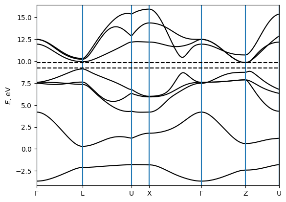
e_vbm_GeTe = np.amax(grid_energy_result.get_data("Energy", 4))
e_cbm_GeTe = np.amin(grid_energy_result.get_data("Energy", 5))
print(f"Valence band maximum : {e_vbm_GeTe:6.3f}")
print(f"Conduction band minimum: {e_cbm_GeTe:6.3f}")
print("VBM k point: ", grid_energy_result.kpoints[np.argmax(grid_energy_result.get_data("Energy", 0))])
print("CBM k point: ", grid_energy_result.kpoints[np.argmin(grid_energy_result.get_data("Energy", 1))])
Minimal symmetric FFT grid :  [3 3 3]
Starting run()
Using the follwing calculators :
############################################################

 'tabulate'  :  <wannierberri.calculators.tabulate.TabulatorAll object at 0x7d998664a9f0>  :
    TabulatorAll - a pack of all k-resolved calculators (Tabulators)

 Includes the following tabulators :
--------------------------------------------------
 "Energy" : <wannierberri.calculators.tabulate.Energy object at 0x7d9bc01b5b50> : calculator not described

--------------------------------------------------

############################################################
Calculation on  grid - checking calculators for compatibility
tabulate <wannierberri.calculators.tabulate.TabulatorAll object at 0x7d998664a9f0>
All calculators are compatible
Grid is regular
The set of k points is a Grid() with NKdiv=[10 10 10], NKFFT=[3 3 3], NKtot=[30 30 30]
generating K_list
Done in 0.0029706954956054688 s
excluding symmetry-equivalent K-points from initial grid
Done in 0.019168615341186523 s
K_list contains 116 Irreducible points(11.6%) out of initial 10x10x10=1000 grid
Done, sum of weights:1.0000000000000007

############################################################
Iteration 0 out of 0
processing 116 K points : using  24 processes.
# K-points calculated  Wall time (sec)  Est. remaining (sec)   Est. total (sec)
time for processing    116 K-points on  24 processes:     0.2470 ; per K-point          0.0021 ; proc-sec per K-point          0.0511
time1 =  7.152557373046875e-07
setting the grid
setting new kpoints
finding equivalent kpoints
collecting
collecting: to_grid  : 0.05633234977722168
collecting: TABresult  : 0.0011496543884277344
collecting - OK : 0.05750703811645508 (2.5033950805664062e-05)
Totally processed 116 K-points
run() finished
setting the grid
setting new kpoints
finding equivalent kpoints
collecting
collecting: to_grid  : 0.04471158981323242
collecting: TABresult  : 0.0009603500366210938
collecting - OK : 0.045702219009399414 (3.0279159545898438e-05)
Valence band maximum   :  9.226
Conduction band minimum:  9.836
VBM k point:  [0.2        0.5        0.76666667]
CBM k point:  [0.  0.  0.5]
[20]:
fig = bands.plot_path_fat(path, close_fig=False, show_fig=False)

ax = fig.get_axes()[0]
ax.axhline(e_vbm_GeTe, c="k", ls="--")
ax.axhline(e_cbm_GeTe, c="k", ls="--")
plt.show(fig)
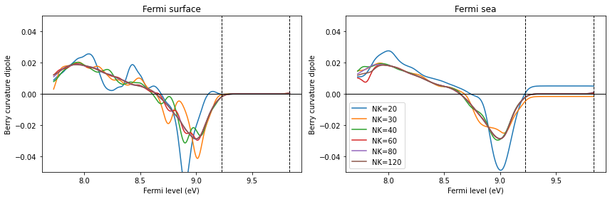
We compute the BCD tensor for the hole-doped case. (The electron-doped case is much harder to converge due to band crossings near the CBM.)
Try to calculate BCD for various grids and compare the convergence of the two methods. (NK=120 will be enough to see convergence.)
[21]:
from wannierberri import calculators as calc
from wannierberri.smoother import FermiDiracSmoother

efermi = np.linspace(e_vbm_GeTe - 1.5, e_cbm_GeTe, 301, True)
smoother = FermiDiracSmoother(efermi, 300.0)

kwargs = dict(
    Efermi=efermi,
    smoother=smoother,
    # kwargs_formula={"external_terms": True},
)

calculators = {
    'berry_dipole_fermi_sea': calc.static.BerryDipole_FermiSea(**kwargs),
    'berry_dipole_fermi_surface': calc.static.BerryDipole_FermiSurf(**kwargs),
}
[22]:
data_GeTe_fsurf_all = {}
data_GeTe_fsea_all = {}

for nk in [20, 30, 40, 60, 80]:
    grid = wberri.Grid(system_GeTe, NK=nk, NKFFT=10)
    result = wberri.run(
        system_GeTe,
        grid=grid,
        calculators=calculators,
        print_Kpoints = False,
        use_irred_kpt = True,
        symmetrize = True,
        restart=False,
    )
    data_GeTe_fsurf_all[nk] = result.results['berry_dipole_fermi_surface'].dataSmooth
    data_GeTe_fsea_all[nk] = result.results['berry_dipole_fermi_sea'].dataSmooth
Starting run()
Using the follwing calculators :
############################################################

 'berry_dipole_fermi_sea'  :  <wannierberri.calculators.static.BerryDipole_FermiSea object at 0x7d9bc82c4b90>  : Berry curvature dipole (dimensionless)

        | With Fermi sea integral. Eq(29) in `Ref <https://www.nature.com/articles/s41524-021-00498-5>`__
        | Output: :math:`D_{\beta\delta} = \int [dk] \partial_\beta \Omega_\delta f`
 'berry_dipole_fermi_surface'  :  <wannierberri.calculators.static.BerryDipole_FermiSurf object at 0x7d9986bea5d0>  : Berry curvature dipole (dimensionless)

        | With Fermi surface integral. Eq(8) in `Ref <https://journals.aps.org/prl/abstract/10.1103/PhysRevLett.115.216806>`__
        | Output: :math:`D_{\beta\delta} = -\int [dk] v_\beta \Omega_\delta f'`
############################################################
Calculation on  grid - checking calculators for compatibility
berry_dipole_fermi_sea <wannierberri.calculators.static.BerryDipole_FermiSea object at 0x7d9bc82c4b90>
berry_dipole_fermi_surface <wannierberri.calculators.static.BerryDipole_FermiSurf object at 0x7d9986bea5d0>
All calculators are compatible
Grid is regular
The set of k points is a Grid() with NKdiv=[2 2 2], NKFFT=[10 10 10], NKtot=[20 20 20]
generating K_list
Done in 4.792213439941406e-05 s
excluding symmetry-equivalent K-points from initial grid
Done in 0.0008957386016845703 s
K_list contains 4 Irreducible points(50.0%) out of initial 2x2x2=8 grid
Done, sum of weights:1.0

############################################################
Iteration 0 out of 0
processing 4 K points : using  24 processes.
# K-points calculated  Wall time (sec)  Est. remaining (sec)   Est. total (sec)
time for processing      4 K-points on  24 processes:     2.5276 ; per K-point          0.6319 ; proc-sec per K-point         15.1655
time1 =  2.384185791015625e-07
Totally processed 4 K-points
run() finished
Starting run()
Using the follwing calculators :
############################################################

 'berry_dipole_fermi_sea'  :  <wannierberri.calculators.static.BerryDipole_FermiSea object at 0x7d9bc82c4b90>  : Berry curvature dipole (dimensionless)

        | With Fermi sea integral. Eq(29) in `Ref <https://www.nature.com/articles/s41524-021-00498-5>`__
        | Output: :math:`D_{\beta\delta} = \int [dk] \partial_\beta \Omega_\delta f`
 'berry_dipole_fermi_surface'  :  <wannierberri.calculators.static.BerryDipole_FermiSurf object at 0x7d9986bea5d0>  : Berry curvature dipole (dimensionless)

        | With Fermi surface integral. Eq(8) in `Ref <https://journals.aps.org/prl/abstract/10.1103/PhysRevLett.115.216806>`__
        | Output: :math:`D_{\beta\delta} = -\int [dk] v_\beta \Omega_\delta f'`
############################################################
Calculation on  grid - checking calculators for compatibility
berry_dipole_fermi_sea <wannierberri.calculators.static.BerryDipole_FermiSea object at 0x7d9bc82c4b90>
berry_dipole_fermi_surface <wannierberri.calculators.static.BerryDipole_FermiSurf object at 0x7d9986bea5d0>
All calculators are compatible
Grid is regular
The set of k points is a Grid() with NKdiv=[3 3 3], NKFFT=[10 10 10], NKtot=[30 30 30]
generating K_list
Done in 0.00021195411682128906 s
excluding symmetry-equivalent K-points from initial grid
Done in 0.002582073211669922 s
K_list contains 6 Irreducible points(22.22%) out of initial 3x3x3=27 grid
Done, sum of weights:1.0

############################################################
Iteration 0 out of 0
processing 6 K points : using  24 processes.
# K-points calculated  Wall time (sec)  Est. remaining (sec)   Est. total (sec)
time for processing      6 K-points on  24 processes:     2.7243 ; per K-point          0.4540 ; proc-sec per K-point         10.8971
time1 =  2.384185791015625e-07
Totally processed 6 K-points
run() finished
Starting run()
Using the follwing calculators :
############################################################

 'berry_dipole_fermi_sea'  :  <wannierberri.calculators.static.BerryDipole_FermiSea object at 0x7d9bc82c4b90>  : Berry curvature dipole (dimensionless)

        | With Fermi sea integral. Eq(29) in `Ref <https://www.nature.com/articles/s41524-021-00498-5>`__
        | Output: :math:`D_{\beta\delta} = \int [dk] \partial_\beta \Omega_\delta f`
 'berry_dipole_fermi_surface'  :  <wannierberri.calculators.static.BerryDipole_FermiSurf object at 0x7d9986bea5d0>  : Berry curvature dipole (dimensionless)

        | With Fermi surface integral. Eq(8) in `Ref <https://journals.aps.org/prl/abstract/10.1103/PhysRevLett.115.216806>`__
        | Output: :math:`D_{\beta\delta} = -\int [dk] v_\beta \Omega_\delta f'`
############################################################
Calculation on  grid - checking calculators for compatibility
berry_dipole_fermi_sea <wannierberri.calculators.static.BerryDipole_FermiSea object at 0x7d9bc82c4b90>
berry_dipole_fermi_surface <wannierberri.calculators.static.BerryDipole_FermiSurf object at 0x7d9986bea5d0>
All calculators are compatible
Grid is regular
The set of k points is a Grid() with NKdiv=[4 4 4], NKFFT=[10 10 10], NKtot=[40 40 40]
generating K_list
Done in 0.0002033710479736328 s
excluding symmetry-equivalent K-points from initial grid
Done in 0.002104520797729492 s
K_list contains 13 Irreducible points(20.31%) out of initial 4x4x4=64 grid
Done, sum of weights:1.0

############################################################
Iteration 0 out of 0
processing 13 K points : using  24 processes.
# K-points calculated  Wall time (sec)  Est. remaining (sec)   Est. total (sec)
time for processing     13 K-points on  24 processes:     4.4277 ; per K-point          0.3406 ; proc-sec per K-point          8.1742
time1 =  0.0
Totally processed 13 K-points
run() finished
Starting run()
Using the follwing calculators :
############################################################

 'berry_dipole_fermi_sea'  :  <wannierberri.calculators.static.BerryDipole_FermiSea object at 0x7d9bc82c4b90>  : Berry curvature dipole (dimensionless)

        | With Fermi sea integral. Eq(29) in `Ref <https://www.nature.com/articles/s41524-021-00498-5>`__
        | Output: :math:`D_{\beta\delta} = \int [dk] \partial_\beta \Omega_\delta f`
 'berry_dipole_fermi_surface'  :  <wannierberri.calculators.static.BerryDipole_FermiSurf object at 0x7d9986bea5d0>  : Berry curvature dipole (dimensionless)

        | With Fermi surface integral. Eq(8) in `Ref <https://journals.aps.org/prl/abstract/10.1103/PhysRevLett.115.216806>`__
        | Output: :math:`D_{\beta\delta} = -\int [dk] v_\beta \Omega_\delta f'`
############################################################
Calculation on  grid - checking calculators for compatibility
berry_dipole_fermi_sea <wannierberri.calculators.static.BerryDipole_FermiSea object at 0x7d9bc82c4b90>
berry_dipole_fermi_surface <wannierberri.calculators.static.BerryDipole_FermiSurf object at 0x7d9986bea5d0>
All calculators are compatible
Grid is regular
The set of k points is a Grid() with NKdiv=[6 6 6], NKFFT=[10 10 10], NKtot=[60 60 60]
generating K_list
Done in 0.0010714530944824219 s
excluding symmetry-equivalent K-points from initial grid
Done in 0.004737138748168945 s
K_list contains 32 Irreducible points(14.81%) out of initial 6x6x6=216 grid
Done, sum of weights:1.0000000000000002

############################################################
Iteration 0 out of 0
processing 32 K points : using  24 processes.
# K-points calculated  Wall time (sec)  Est. remaining (sec)   Est. total (sec)
                  24              6.5                   2.2                   8.7
time for processing     32 K-points on  24 processes:     7.8472 ; per K-point          0.2452 ; proc-sec per K-point          5.8854
time1 =  2.384185791015625e-07
Totally processed 32 K-points
run() finished
Starting run()
Using the follwing calculators :
############################################################

 'berry_dipole_fermi_sea'  :  <wannierberri.calculators.static.BerryDipole_FermiSea object at 0x7d9bc82c4b90>  : Berry curvature dipole (dimensionless)

        | With Fermi sea integral. Eq(29) in `Ref <https://www.nature.com/articles/s41524-021-00498-5>`__
        | Output: :math:`D_{\beta\delta} = \int [dk] \partial_\beta \Omega_\delta f`
 'berry_dipole_fermi_surface'  :  <wannierberri.calculators.static.BerryDipole_FermiSurf object at 0x7d9986bea5d0>  : Berry curvature dipole (dimensionless)

        | With Fermi surface integral. Eq(8) in `Ref <https://journals.aps.org/prl/abstract/10.1103/PhysRevLett.115.216806>`__
        | Output: :math:`D_{\beta\delta} = -\int [dk] v_\beta \Omega_\delta f'`
############################################################
Calculation on  grid - checking calculators for compatibility
berry_dipole_fermi_sea <wannierberri.calculators.static.BerryDipole_FermiSea object at 0x7d9bc82c4b90>
berry_dipole_fermi_surface <wannierberri.calculators.static.BerryDipole_FermiSurf object at 0x7d9986bea5d0>
All calculators are compatible
Grid is regular
The set of k points is a Grid() with NKdiv=[8 8 8], NKFFT=[10 10 10], NKtot=[80 80 80]
generating K_list
Done in 0.0015788078308105469 s
excluding symmetry-equivalent K-points from initial grid
Done in 0.012530088424682617 s
K_list contains 65 Irreducible points(12.7%) out of initial 8x8x8=512 grid
Done, sum of weights:1.0

############################################################
Iteration 0 out of 0
processing 65 K points : using  24 processes.
# K-points calculated  Wall time (sec)  Est. remaining (sec)   Est. total (sec)
                  24              6.7                  11.4                  18.1
                  48             12.7                   4.5                  17.2
time for processing     65 K-points on  24 processes:    14.9988 ; per K-point          0.2308 ; proc-sec per K-point          5.5380
time1 =  2.384185791015625e-07
Totally processed 65 K-points
run() finished
[23]:
nk = 20
print("Shape of data: ", data_GeTe_fsurf_all[nk].shape)

print("Maximum value for each components (Fermi surface): ")
print(np.amax(abs(data_GeTe_fsurf_all[nk]), axis=0))

print("Maximum value for each components (Fermi sea): ")
print(np.amax(abs(data_GeTe_fsea_all[nk]), axis=0))
Shape of data:  (301, 3, 3)
Maximum value for each components (Fermi surface):
[[5.51672243e-20 4.60776297e-02 3.24189788e-19]
 [4.60776297e-02 5.39827954e-20 7.13428333e-20]
 [4.98219278e-19 6.56821114e-20 5.19808344e-21]]
Maximum value for each components (Fermi sea):
[[4.54791197e-19 4.41044006e-02 3.46994105e-18]
 [4.41044006e-02 8.31504010e-20 4.67009595e-19]
 [1.79557219e-19 5.06406370e-20 3.38813179e-21]]
Let us focus on the undoped case: Fermi level between the VBM and the CBM. Then, $:nbsphinx-math:frac{partial}{partial k^a} f_0 (\varepsilon_{n:nbsphinx-math:mathbf{k}}) =0 $ holds so that the BCD is always 0. For the Fermi surface method, the integrand is 0 at every k point, so the integral is also 0. However, for the Fermi sea method, the integrand is not 0, and the integral becomes 0 only due to a calculation.
[24]:
ic = 0
fig, axes = plt.subplots(1, 2, figsize=(12, 4))
for nk in sorted(list(data_GeTe_fsurf_all.keys())):
    c = f"C{ic}"
    axes[0].plot(efermi, data_GeTe_fsurf_all[nk][:, 0, 1], c=c, label=f"NK={nk}")
    axes[1].plot(efermi, data_GeTe_fsea_all[nk][:, 0, 1], c=c, label=f"NK={nk}")
    ic += 1

axes[0].set_title("Fermi surface")
axes[1].set_title("Fermi sea")

for ax in axes:
    ax.axhline(0, c="k", lw=1)
    ax.axvline(e_vbm_GeTe, c="k", lw=1, ls="--")
    ax.axvline(e_cbm_GeTe, c="k", lw=1, ls="--")
    ax.set_xlabel("Fermi level (eV)")
    ax.set_ylabel("Berry curvature dipole")
    ax.set_ylim(np.array([-0.01, 0.03]) * 1)
    ax.set_xlim([e_vbm_GeTe - 0.1, e_cbm_GeTe + 0.1])

axes[1].legend()
fig.suptitle("zoom around the band gap")
plt.tight_layout()
plt.show()
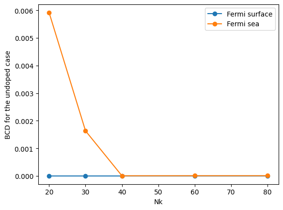
[25]:
# Choose the Fermi level index at the middle of the band gap.
ifermi = np.argmin(np.abs(efermi - (e_vbm_GeTe + e_cbm_GeTe) / 2))

nklist = sorted(list(data_GeTe_fsurf_all.keys()))

print("D_xy for the undoped case")
print("NK : ", nklist)
print("Fermi sea: ", [data_GeTe_fsea_all[nk][ifermi, 0, 1] for nk in nklist])
print("Fermi surface: ", [data_GeTe_fsurf_all[nk][ifermi, 0, 1] for nk in nklist])

plt.plot(nklist, [np.abs(data_GeTe_fsurf_all[NK][ifermi, 0, 1]) for NK in nklist], "o-", label="Fermi surface")
plt.plot(nklist, [abs(data_GeTe_fsea_all[NK][ifermi, 0, 1]) for NK in nklist], "o-", label="Fermi sea")
plt.legend()
# plt.yscale("log") # Also try logscale
plt.xlabel("Nk")
plt.ylabel("BCD for the undoped case")
plt.show()
D_xy for the undoped case
NK :  [20, 30, 40, 60, 80]
Fermi sea:  [np.float64(0.0059157091071223725), np.float64(-0.0016322918511831538), np.float64(-6.155505721592083e-06), np.float64(8.172893691772796e-06), np.float64(8.74329391690673e-06)]
Fermi surface:  [np.float64(0.0), np.float64(0.0), np.float64(0.0), np.float64(0.0), np.float64(0.0)]
Further questions
If you are interested, try to answer the following questions: - What happens if one uses an un-symmetrized model? Does Fermi sea BCD with the Fermi energy inside the gap converge to 0? - What happens if one uses the tetrahedron method? - What happens for the zero-temperature case (you may use .data instead of .dataSmooth)?