DIY tutorial
As we learned from the basic tutorial, in WannierBerri calculations are done by `Calculator <https://wannier-berri.org/docs/calculators.html#wannierberri.calculators.Calculator>`__s. In this tutorial we will se how to create our own calculators.
As an example let’s consider anomalous Nernst conductivity (Xiao et al. 2006 ). In the zero-temperature limit \(\alpha_{\alpha\beta}^{\rm ANE}\) may be obtained from AHC \(\sigma_{\alpha\beta}(\epsilon)^{\rm AHE}\) evaluated over a dense grid of Fermi levels \(\epsilon\)
where \(f(\varepsilon)=1/\left(1+e^\frac{\varepsilon-\mu}{k_{\rm B}T}\right)\) and the AHC is defined as a Fermi-sea integral of Berry curvature
\begin{equation} \sigma^{\rm AHC}_{xy} = -\frac{e^2}{\hbar} \sum_n \int\frac{d\mathbf{k}}{(2\pi)^3} \Omega^n_\gamma f(\epsilon_n) \label{eq:ahc}\tag{2} \end{equation}
In the zero-temperature limit it reduced to
Where we omit the dimensional factor for simplicity.
Thus, there are two ways of calculating ANE : * via eq (\ref{eq:ane-ahc}) * via eq (\ref{eq:ane})
let’s try eq (\ref{eq:ane-ahc}) first, because AHC is already implemented
Warning : this is an advanced tutorial. You something may not work from first try, you need to work with documentation to resolve the problem, but do not hesitate to ask the TA if you cannot.
[3]:
# Preliminary

# Set environment variables - not mandatory but recommended if you use Parallel()
#import os
#os.environ['OPENBLAS_NUM_THREADS'] = '1'
#os.environ['MKL_NUM_THREADS'] = '1'


import wannierberri as wberri
import wannierberri.models
print (f"Using WannierBerri version {wberri.__version__}")
import numpy as np
import matplotlib.pyplot as plt

import ray
ray.init(num_cpus=16, ignore_reinit_error=True)
2026-03-30 23:57:28,390 INFO worker.py:1765 -- Calling ray.init() again after it has already been called.
Using WannierBerri version 26.3.3.dev2+g2858c459a
[3]:
| Python version: | 3.12.12 |
| Ray version: | 2.48.0 |
| Dashboard: | http://127.0.0.1:8268 |
[4]:
# Instead of Wannier functions, we work with a Hlldane model here https://wannier-berri.org/docs/models.html

model=wberri.models.Haldane_ptb()
system = wberri.System_R.from_pythtb(model)
Reading the system from PythTB model. Needed data: {'Ham'}
number of wannier functions: 2
shape of Ham_R = (7, 2, 2)
Real-space lattice:
 [[1.        0.        0.       ]
 [0.5       0.8660254 0.       ]
 [0.        0.        1.       ]]
Number of wannier functions: 2
Number of R points: 7
Recommended size of FFT grid [3 3 1]
Reading the system from PythTB finished successfully
anomalous Hall conductivity
Now, let’s evaluate the AHC on a grid of Ef-points, and then take a derivtive
[5]:
calculators = {}
Efermi = np.linspace(-3,3,21)
# Set a grid
grid = wberri.Grid(system, length=30 )   # length [ Ang] ~= 2*pi/dk

calculators ["ahc"] = wberri.calculators.static.AHC(Efermi=Efermi,
                                                    tetra=True,
                                                    constant_factor=1,
                                                    kwargs_formula={"external_terms":False})

result_run_ahc = wberri.run(system,
            grid=grid,
            calculators = calculators,
            adpt_num_iter=0,
            fout_name='Fe',
            )
Minimal symmetric FFT grid :  [3 3 1]
Starting run()
Using the follwing calculators :
############################################################

 'ahc'  :  <wannierberri.calculators.static.AHC object at 0x7995067ac1a0>  : Anomalous Hall conductivity (:math:`s^3 \cdot A^2 / (kg \cdot m^3) = S/m`)

        | With Fermi sea integral Eq(11) in `Ref <https://www.nature.com/articles/s41524-021-00498-5>`__
        | Output: :math:`O = -e^2/\hbar \int [dk] \Omega f`
        | Instruction: :math:`j_\alpha = \sigma_{\alpha\beta} E_\beta = \epsilon_{\alpha\beta\delta} O_\delta E_\beta`
############################################################
Calculation on  grid - checking calculators for compatibility
ahc <wannierberri.calculators.static.AHC object at 0x7995067ac1a0>
All calculators are compatible
Grid is regular
The set of k points is a Grid() with NKdiv=[7 7 1], NKFFT=[5 5 1], NKtot=[35 35  1]
generating K_list
Done in 0.0001990795135498047 s
excluding symmetry-equivalent K-points from initial grid
Done in 0.0007872581481933594 s
K_list contains 49 Irreducible points(100.0%) out of initial 7x7x1=49 grid
Done, sum of weights:1.0000000000000007

############################################################
Iteration 0 out of 0
processing 49 K points : using  16 processes.
# K-points calculated  Wall time (sec)  Est. remaining (sec)   Est. total (sec)
                  48              5.2                   0.1                   5.3
time for processing     49 K-points on  16 processes:     5.2444 ; per K-point          0.1070 ; proc-sec per K-point          1.7124
time1 =  2.384185791015625e-07
Totally processed 49 K-points
run() finished
[6]:
!ls
Fe-ahc_iter-0000.dat  Fe-ane_iter-0000.npz            tutorial-wb-DIY.ipynb
Fe-ahc_iter-0000.npz  Klist_ahc.pickle
Fe-ane_iter-0000.dat  tutorial-wb-DIY-solution.ipynb
[7]:
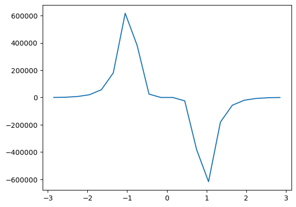
# taking derivative and plotting

ef = result_run_ahc.results["ahc"].Energies[0]
ahc_z = result_run_ahc.results["ahc"].data[:,2]

# take the derivative
d_ef=ef[1]-ef[0]
d_ahc_z = (ahc_z[1:]-ahc_z[:-1])/d_ef
efnew = (ef[1:]+ef[:-1])/2

plt.plot(efnew, d_ahc_z)
[7]:
[<matplotlib.lines.Line2D at 0x7994fd165850>]
Look into documentation
Look into documentation to see how the AHC calculator is defined : look for “Calculator” on https://docs.wannier-berri.org and press the “source” link.
One can see that it is based on the StaticCalculator, and only redefines the __init__ method. Namely, it redefines formula that stands under the integral (Berry curvature) and fder=0 meaning that the formula is weighted by the 0th derivative of the Fermi distribution.
copy the definition of AHC calculator and redefine the and below and define the init class
(hint : leave the factor the same, for simplicity) (hint : formula shouldbe imported from wannierberri.formula.covariant.DerOmega )
[8]:
from wannierberri.calculators.static import StaticCalculator
from wannierberri.formula.covariant import Omega
from wannierberri import factors


class ANC(StaticCalculator):
    r"""Anomalous Nernst conductivity

        | Output: :math:`O = \int [dk] \Omega f' `
        """

    def __init__(self,
                 constant_factor=1, # Figure out the pre-factor yourself
                 **kwargs):
        """describe input parameters here"""
        self.Formula = Omega
        self.fder = 1
        super().__init__(constant_factor=constant_factor, **kwargs)
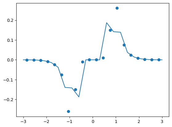
Evaluate ANE using the new calculator and plot the result
[9]:
# insert the needed code below

calculators = {}
# Set a grid
grid = wberri.Grid(system, length=50 )   # length [ Ang] ~= 2*pi/dk

calculators ["ane"] = ANC(Efermi=Efermi,tetra=True)

result_run_ane = wberri.run(system,
            grid=grid,
            calculators = calculators,
            adpt_num_iter=0,
            fout_name='Fe',
            restart=False,
            )
Minimal symmetric FFT grid :  [3 3 1]
Starting run()
Using the follwing calculators :
############################################################

 'ane'  :  <__main__.ANC object at 0x7994fe8d3230>  : Anomalous Nernst conductivity

        | Output: :math:`O = \int [dk] \Omega f' `

############################################################
Calculation on  grid - checking calculators for compatibility
ane <__main__.ANC object at 0x7994fe8d3230>
All calculators are compatible
Grid is regular
The set of k points is a Grid() with NKdiv=[19 19  1], NKFFT=[3 3 1], NKtot=[57 57  1]
generating K_list
Done in 0.001165628433227539 s
excluding symmetry-equivalent K-points from initial grid
Done in 0.00506138801574707 s
K_list contains 361 Irreducible points(100.0%) out of initial 19x19x1=361 grid
Done, sum of weights:0.999999999999993

############################################################
Iteration 0 out of 0
processing 361 K points : using  16 processes.
# K-points calculated  Wall time (sec)  Est. remaining (sec)   Est. total (sec)
/home/stepan/github/wannier-berri/wannierberri/grid/grid.py:260: UserWarning:  the requested k-grid [58 58 50] was adjusted to [57 57 50].
  warnings.warn(f" the requested k-grid {NK} was adjusted to {NKFFT * NKdiv}. ")
time for processing    361 K-points on  16 processes:     0.3200 ; per K-point          0.0009 ; proc-sec per K-point          0.0142
time1 =  4.76837158203125e-07
Totally processed 361 K-points
run() finished
[10]:
ef = result_run_ane.results["ane"].Energies[0]
ane_z = result_run_ane.results["ane"].dataSmooth[:,2]


plt.scatter(efnew,d_ahc_z)
plt.plot(ef, ane_z)
plt.show()
Questions:
Make the k-points or Efermi denser. Will the agreement improve?
we calculated the AHC and ANE with zero refinement iterations, and the results matched well (or at least they should). If we calculate them separately, but with some refinement iterations, will the results match?
What if we use refinement itrations and run the two calculations together, in one
run()call ?
FormulaProduct
Look at the definition of erryDipole_FermiSurf
https://wannier-berri.org/_modules/wannierberri/calculators/static.html
It evaluates
\begin{equation} D_{ab} =\sum_n \int\frac{d\mathbf{k}}{(2\pi)^3} v_a\Omega^n_b f(\epsilon_n) \label{eq:ahc}\tag{2} \end{equation}
also look at definition of the Feormula https://wannier-berri.org/docs/formula.html
you can see that it is base on a FormulaProduct. Essentially, by analogy you may define any tensor, e.g.
i.e. product of several quantities weighted by rge second derivative of Fermi distribution. You may write any analogous formula, if you want. Try to define corresponding FormulaProduct and StaticCalculator classes, and try to evaluate them.
[ ]:
[ ]:
Problem :
try to prove (analytically and numerically) that
and tell me what is the factor missing?
** Have fun ! **
[ ]: