Symmetrization of Wannier Hamiltonian and matrices
By Xiaoxiong Liu : xxliu@physik.uzh.ch
The real-space Wannier Hamiltonian obtained by Wannier90 code generally does not strictly preserve the corresponding symmetry. The slight loss of symmetry will gap the expected band intersections. Berry curvature and orbital magnetic moment are more sensitive to symmetry than energy eigenvalues. In the following, I give details about the symmetrization of Wannier Hamiltonian and matrices.
In WannierBerri, our built-in symmetrization method can enforce symmetrizing Wannier Hamiltonian (Ham_R) and matrices (AA_R, BB_R, CC_R, SS_R) after reading them.
\(\texttt{Ham\_R} = <n0|\hat{H}|mR>\)
\(\texttt{AA\_R} = <n0|\hat{r}|mR>\)
\(\texttt{BB\_R} = <n0|\hat{H}\cdot(\hat{r}-\hat{R})|mR>\)
\(\texttt{CC\_Rc} = i \epsilon_{abc} <n0|\hat{r}_a\cdot\hat{H}\cdot(\hat{r}_b-\hat{R}_b)|mR>\)
\(\texttt{SS\_R} = <n0|\hat{\sigma}|mR>\)
They are needed when calculating different quantities: 1. Energy eigenvalue <– Ham_R 2. Berry Curvature <– Ham_R, AA_R 3. Orbital magnetic moment <– Ham_R, AA_R, BB_R, CC_R 4. Spin magnetic moment <– SS_R
NOTE: This method only works with Wannier Hamiltonian without maximal localized.
We will show you two examples: 1. Symmetrize nonmagnetic system with SOC (trigonal Te) 2. Symmetrize magnetic system with SOC (bcc Fe)
[1]:
#import necessary packages
import wannierberri as wberri
import warnings
tested_version = '1.3.0'
if wberri.__version__ != tested_version:
    warnings.warn(f'This tutorial was tested with version {tested_version} of wannierberri. You are using version {wberri.__version__}.')


import numpy as np
import matplotlib.pyplot as plt #for plotting figures

import ray
ray.init(num_cpus=16) # initialize ray for parallelization
/home/stepan/github/WannierBerri-tutorial/.conda/lib/python3.12/site-packages/tqdm/auto.py:21: TqdmWarning: IProgress not found. Please update jupyter and ipywidgets. See https://ipywidgets.readthedocs.io/en/stable/user_install.html
  from .autonotebook import tqdm as notebook_tqdm
2026-03-31 00:05:25,854 INFO util.py:154 -- Missing packages: ['ipywidgets']. Run `pip install -U ipywidgets`, then restart the notebook server for rich notebook output.
/tmp/ipykernel_89047/879675732.py:6: UserWarning: This tutorial was tested with version 1.3.0 of wannierberri. You are using version 26.3.3.dev2+g2858c459a.
  warnings.warn(f'This tutorial was tested with version {tested_version} of wannierberri. You are using version {wberri.__version__}.')
2026-03-31 00:05:28,028 INFO worker.py:1918 -- Started a local Ray instance. View the dashboard at http://127.0.0.1:8267
[1]:
| Python version: | 3.12.12 |
| Ray version: | 2.48.0 |
| Dashboard: | http://127.0.0.1:8267 |
Nonmagnetic system (trigonal Te)
[2]:
#Reading Wannier Hamiltonian and position element matrix from Te_tb.dat file.
#We bulit to system, `system_Te` without symmetrization and `system_Te_sym` with symmetrization

import copy

from irrep.spacegroup import SpaceGroup
from wannierberri.symmetry.sawf import SymmetrizerSAWF
from wannierberri.symmetry.projections import Projection


system_Te=wberri.System_R.from_tb_dat(tb_file='./Te_data/Te_tb.dat',berry=True)
system_Te.spin_block2interlace()  # the data come from old vasp, which stored WF spins separated into two blocks. QE and modern VASP intrelace the spin channels

#Check unsymmetrized system
system = system_Te

def check_onsite(system):
    #find index of R=[0,0,0] in R-vector list
    #dimension of Hamiltonian is [num_wann, num_wann, num_Rvec]
    iR0 = system.rvec.iR0
    onsite_Te_1 = np.diagonal(system.Ham_R[iR0]).real[:2]
    onsite_Te_2 = np.diagonal(system.Ham_R[iR0]).real[2:4]
    print(f'on-site energy of Te_1 orbitals spin up : {onsite_Te_1[0]}, spin_down: {onsite_Te_1[1]}, difference: {abs(onsite_Te_1[0]-onsite_Te_1[1])}')
    print(f'on-site energy of Te_2 orbitals spin up : {onsite_Te_2[0]}, spin_down: {onsite_Te_2[1]}, difference: {abs(onsite_Te_2[0]-onsite_Te_2[1])}')
    print('difference:', abs(onsite_Te_1-onsite_Te_2))

print('unsymmetrized')
check_onsite(system_Te)
reading TB file ./Te_data/Te_tb.dat ( written on  9May2022 at 22:54:49 )
Real-space lattice:
 [[ 4.457      0.         0.       ]
 [-2.2285     3.8598752  0.       ]
 [ 0.         0.         5.9581176]]
Number of wannier functions: 24
Number of R points: 195
Recommended size of FFT grid [7 9 5]
Reading the system from ./Te_data/Te_tb.dat finished successfully
unsymmetrized
on-site energy of Te_1 orbitals spin up : -5.585966, spin_down: -5.5859776, difference: 1.1599999999667432e-05
on-site energy of Te_2 orbitals spin up : -5.588091, spin_down: -5.5880802, difference: 1.0800000000088517e-05
difference: [0.002125  0.0021026]
[20]:
system_Te_sym_new=wberri.System_R.from_tb_dat(tb_file='./Te_data/Te_tb.dat',berry=True)
system_Te_sym_new.spin_block2interlace()  # the data come from old vasp, which stored WF spins separated into two blocks. QE and modern VASP intrelace the spin channels


# #symmetrization step - new method using SymmetrizerSAWF
x = 0.274
positions = np.array([ [x , x  ,   0.],
                      [1-x, 0  , 1./3],
                      [0  , 1-x, 2./3]] )

spacegroup = SpaceGroup.from_cell(real_lattice=system_Te.real_lattice,
                                  positions=positions,
                                  typat=[1,1,1],
                                     magmom=None, include_TR=True,
                                     spinor=True)
spacegroup.show()

proj_list = []
for proj_str in ["s","p"]:
        proj = Projection(position_num=positions, orbital=proj_str, spacegroup=spacegroup, rotate_basis=False)
        # In the win file all projections were defined without xaxis/zaxis rotation, so we set rotate_basis=False.
        # print (f"adding projection {proj} ({pos} {suborbital})")
        proj_list.append(proj)
symmetrizer = SymmetrizerSAWF.from_spacegroup_and_projections(spacegroup=spacegroup, projections=proj_list)
system_Te_sym_new.symmetrize2(symmetrizer)


print('symmetrized')
check_onsite(system_Te_sym_new)
reading TB file ./Te_data/Te_tb.dat ( written on  9May2022 at 22:54:49 )
Real-space lattice:
 [[ 4.457      0.         0.       ]
 [-2.2285     3.8598752  0.       ]
 [ 0.         0.         5.9581176]]
Number of wannier functions: 24
Number of R points: 195
Recommended size of FFT grid [7 9 5]
Reading the system from ./Te_data/Te_tb.dat finished successfully


 ---------- CRYSTAL STRUCTURE ----------


Cell vectors in angstroms:

      Vectors of DFT cell
a0 =  4.4570   0.0000   0.0000
a1 = -2.2285   3.8599   0.0000
a2 =  0.0000   0.0000   5.9581


 ---------- SPACE GROUP -----------


Space group: P3_1211' (# 152.34)
Number of symmetries: 12 (mod. lattice translations)

 ### 1

rotation : |  1   0   0 |
           |  0   1   0 |
           |  0   0   1 |


 gk = [kx, ky, kz]

spinor rot.         : | 1.000+0.000j  0.000+0.000j |
                      | 0.000+0.000j  1.000+0.000j |

translation         :  [   0.0000   0.0000   0.0000 ]

axis: [0. 0. 1.] ; angle =  0 , inversion: False, time reversal: False

 ### 2

rotation : |  1   0   0 |
           |  0   1   0 |
           |  0   0   1 |


 gk = [-kx, -ky, -kz]

spinor rot.         : | 1.000+0.000j  0.000+0.000j |
                      | 0.000+0.000j  1.000+0.000j |

translation         :  [   0.0000   0.0000   0.0000 ]

axis: [0. 0. 1.] ; angle =  0 , inversion: False, time reversal: True

 ### 3

rotation : |  0  -1   0 |
           |  1  -1   0 |
           |  0   0   1 |


 gk = [-kx-ky, kx, kz]

spinor rot.         : | 0.500-0.866j  0.000+0.000j |
                      | 0.000+0.000j  0.500+0.866j |

translation         :  [   0.0000   0.0000   0.3333 ]

axis: [0. 0. 1.] ; angle = 2/3 pi, inversion: False, time reversal: False

 ### 4

rotation : |  0  -1   0 |
           |  1  -1   0 |
           |  0   0   1 |


 gk = [kx+ky, -kx, -kz]

spinor rot.         : | 0.500-0.866j  0.000+0.000j |
                      | 0.000+0.000j  0.500+0.866j |

translation         :  [   0.0000   0.0000   0.3333 ]

axis: [0. 0. 1.] ; angle = 2/3 pi, inversion: False, time reversal: True

 ### 5

rotation : | -1   1   0 |
           | -1   0   0 |
           |  0   0   1 |


 gk = [ky, -kx-ky, kz]

spinor rot.         : | 0.500+0.866j  0.000+0.000j |
                      | 0.000+0.000j  0.500-0.866j |

translation         :  [   0.0000   0.0000   0.6667 ]

axis: [0. 0. 1.] ; angle = -2/3 pi, inversion: False, time reversal: False

 ### 6

rotation : | -1   1   0 |
           | -1   0   0 |
           |  0   0   1 |


 gk = [-ky, kx+ky, -kz]

spinor rot.         : | 0.500+0.866j  0.000+0.000j |
                      | 0.000+0.000j  0.500-0.866j |

translation         :  [   0.0000   0.0000   0.6667 ]

axis: [0. 0. 1.] ; angle = -2/3 pi, inversion: False, time reversal: True

 ### 7

rotation : |  0   1   0 |
           |  1   0   0 |
           |  0   0  -1 |


 gk = [ky, kx, -kz]

spinor rot.         : | 0.000+0.000j  0.866+0.500j |
                      |-0.866+0.500j  0.000-0.000j |

translation         :  [   0.0000   0.0000   0.0000 ]

axis: [-0.5      -0.866025  0.      ] ; angle = 1 pi, inversion: False, time reversal: False

 ### 8

rotation : |  0   1   0 |
           |  1   0   0 |
           |  0   0  -1 |


 gk = [-ky, -kx, kz]

spinor rot.         : | 0.000+0.000j  0.866+0.500j |
                      |-0.866+0.500j  0.000-0.000j |

translation         :  [   0.0000   0.0000   0.0000 ]

axis: [-0.5      -0.866025  0.      ] ; angle = 1 pi, inversion: False, time reversal: True

 ### 9

rotation : |  1  -1   0 |
           |  0  -1   0 |
           |  0   0  -1 |


 gk = [kx, -kx-ky, -kz]

spinor rot.         : | 0.000+0.000j  0.000-1.000j |
                      | 0.000-1.000j  0.000+0.000j |

translation         :  [   0.0000   0.0000   0.6667 ]

axis: [1. 0. 0.] ; angle = 1 pi, inversion: False, time reversal: False

 ### 10

rotation : |  1  -1   0 |
           |  0  -1   0 |
           |  0   0  -1 |


 gk = [-kx, kx+ky, kz]

spinor rot.         : | 0.000+0.000j  0.000-1.000j |
                      | 0.000-1.000j  0.000+0.000j |

translation         :  [   0.0000   0.0000   0.6667 ]

axis: [1. 0. 0.] ; angle = 1 pi, inversion: False, time reversal: True

 ### 11

rotation : | -1   0   0 |
           | -1   1   0 |
           |  0   0  -1 |


 gk = [-kx-ky, ky, -kz]

spinor rot.         : | 0.000+0.000j  0.866-0.500j |
                      |-0.866-0.500j  0.000+0.000j |

translation         :  [   0.0000   0.0000   0.3333 ]

axis: [ 0.5      -0.866025  0.      ] ; angle = 1 pi, inversion: False, time reversal: False

 ### 12

rotation : | -1   0   0 |
           | -1   1   0 |
           |  0   0  -1 |


 gk = [kx+ky, -ky, kz]

spinor rot.         : | 0.000+0.000j  0.866-0.500j |
                      |-0.866-0.500j  0.000+0.000j |

translation         :  [   0.0000   0.0000   0.3333 ]

axis: [ 0.5      -0.866025  0.      ] ; angle = 1 pi, inversion: False, time reversal: True
num_blocks_left = 2, num_blocks_right = 2
number o R-vectors before symmetrization: 195
number o R-vectors after symmetrization: 483
symmetrized
on-site energy of Te_1 orbitals spin up : -5.586680166666666, spin_down: -5.586680166666666, difference: 0.0
on-site energy of Te_2 orbitals spin up : -5.586680166666666, spin_down: -5.586680166666666, difference: 0.0
difference: [0. 0.]
[21]:
#Symmetrization step (old method interface, but still works so far. Internally it creates a SymmetrizerSAWF object)
system_Te_sym_old=copy.deepcopy(system_Te)
system_Te_sym_old.symmetrize(
    # positions: positions of each atoms in a unitcell (direct coordinate system)
    positions = positions,
    # atom_name: name of each atoms, need to correspond to position order.
    atom_name = ['Te','Te','Te'],
    # projections: should be the same with projection card in wannier90.win
    proj = ['Te:s','Te:p'],
    # soc: with soc or spinless
    soc=True,
    )

print('symmetrized - old interface')
check_onsite(system_Te_sym_old)
 ---------- CRYSTAL STRUCTURE ----------


Cell vectors in angstroms:

      Vectors of DFT cell
a0 =  4.4570   0.0000   0.0000
a1 = -2.2285   3.8599   0.0000
a2 =  0.0000   0.0000   5.9581


 ---------- SPACE GROUP -----------


Space group: P3_1211' (# 152.34)
Number of symmetries: 12 (mod. lattice translations)

 ### 1

rotation : |  1   0   0 |
           |  0   1   0 |
           |  0   0   1 |


 gk = [kx, ky, kz]

spinor rot.         : | 1.000+0.000j  0.000+0.000j |
                      | 0.000+0.000j  1.000+0.000j |

translation         :  [   0.0000   0.0000   0.0000 ]

axis: [0. 0. 1.] ; angle =  0 , inversion: False, time reversal: False

 ### 2

rotation : |  1   0   0 |
           |  0   1   0 |
           |  0   0   1 |


 gk = [-kx, -ky, -kz]

spinor rot.         : | 1.000+0.000j  0.000+0.000j |
                      | 0.000+0.000j  1.000+0.000j |

translation         :  [   0.0000   0.0000   0.0000 ]

axis: [0. 0. 1.] ; angle =  0 , inversion: False, time reversal: True

 ### 3

rotation : |  0  -1   0 |
           |  1  -1   0 |
           |  0   0   1 |


 gk = [-kx-ky, kx, kz]

spinor rot.         : | 0.500-0.866j  0.000+0.000j |
                      | 0.000+0.000j  0.500+0.866j |

translation         :  [   0.0000   0.0000   0.3333 ]

axis: [0. 0. 1.] ; angle = 2/3 pi, inversion: False, time reversal: False

 ### 4

rotation : |  0  -1   0 |
           |  1  -1   0 |
           |  0   0   1 |


 gk = [kx+ky, -kx, -kz]

spinor rot.         : | 0.500-0.866j  0.000+0.000j |
                      | 0.000+0.000j  0.500+0.866j |

translation         :  [   0.0000   0.0000   0.3333 ]

axis: [0. 0. 1.] ; angle = 2/3 pi, inversion: False, time reversal: True

 ### 5

rotation : | -1   1   0 |
           | -1   0   0 |
           |  0   0   1 |


 gk = [ky, -kx-ky, kz]

spinor rot.         : | 0.500+0.866j  0.000+0.000j |
                      | 0.000+0.000j  0.500-0.866j |

translation         :  [   0.0000   0.0000   0.6667 ]

axis: [0. 0. 1.] ; angle = -2/3 pi, inversion: False, time reversal: False

 ### 6

rotation : | -1   1   0 |
           | -1   0   0 |
           |  0   0   1 |


 gk = [-ky, kx+ky, -kz]

spinor rot.         : | 0.500+0.866j  0.000+0.000j |
                      | 0.000+0.000j  0.500-0.866j |

translation         :  [   0.0000   0.0000   0.6667 ]

axis: [0. 0. 1.] ; angle = -2/3 pi, inversion: False, time reversal: True

 ### 7

rotation : |  0   1   0 |
           |  1   0   0 |
           |  0   0  -1 |


 gk = [ky, kx, -kz]

spinor rot.         : | 0.000+0.000j  0.866+0.500j |
                      |-0.866+0.500j  0.000-0.000j |

translation         :  [   0.0000   0.0000   0.0000 ]

axis: [-0.5      -0.866025  0.      ] ; angle = 1 pi, inversion: False, time reversal: False

 ### 8

rotation : |  0   1   0 |
           |  1   0   0 |
           |  0   0  -1 |


 gk = [-ky, -kx, kz]

spinor rot.         : | 0.000+0.000j  0.866+0.500j |
                      |-0.866+0.500j  0.000-0.000j |

translation         :  [   0.0000   0.0000   0.0000 ]

axis: [-0.5      -0.866025  0.      ] ; angle = 1 pi, inversion: False, time reversal: True

 ### 9

rotation : |  1  -1   0 |
           |  0  -1   0 |
           |  0   0  -1 |


 gk = [kx, -kx-ky, -kz]

spinor rot.         : | 0.000+0.000j  0.000-1.000j |
                      | 0.000-1.000j  0.000+0.000j |

translation         :  [   0.0000   0.0000   0.6667 ]

axis: [1. 0. 0.] ; angle = 1 pi, inversion: False, time reversal: False

 ### 10

rotation : |  1  -1   0 |
           |  0  -1   0 |
           |  0   0  -1 |


 gk = [-kx, kx+ky, kz]

spinor rot.         : | 0.000+0.000j  0.000-1.000j |
                      | 0.000-1.000j  0.000+0.000j |

translation         :  [   0.0000   0.0000   0.6667 ]

axis: [1. 0. 0.] ; angle = 1 pi, inversion: False, time reversal: True

 ### 11

rotation : | -1   0   0 |
           | -1   1   0 |
           |  0   0  -1 |


 gk = [-kx-ky, ky, -kz]

spinor rot.         : | 0.000+0.000j  0.866-0.500j |
                      |-0.866-0.500j  0.000+0.000j |

translation         :  [   0.0000   0.0000   0.3333 ]

axis: [ 0.5      -0.866025  0.      ] ; angle = 1 pi, inversion: False, time reversal: False

 ### 12

rotation : | -1   0   0 |
           | -1   1   0 |
           |  0   0  -1 |


 gk = [kx+ky, -ky, kz]

spinor rot.         : | 0.000+0.000j  0.866-0.500j |
                      |-0.866-0.500j  0.000+0.000j |

translation         :  [   0.0000   0.0000   0.3333 ]

axis: [ 0.5      -0.866025  0.      ] ; angle = 1 pi, inversion: False, time reversal: True
pos_list: [[0, 1, 2]]
proj: Projection 0.274, 0.274, 0.0:['s'] with 6 Wannier functions (3 per spin x2 spins)
 on 3 points (2 per site)
orbital = s, num wann per site = 2
pos_list: [[0, 1, 2]]
proj: Projection 0.274, 0.274, 0.0:['p'] with 18 Wannier functions (9 per spin x2 spins)
 on 3 points (6 per site)
orbital = p, num wann per site = 6
new_wann_indices: [0, 1, 2, 3, 4, 5, 6, 7, 8, 9, 10, 11, 12, 13, 14, 15, 16, 17, 18, 19, 20, 21, 22, 23]
num_blocks_left = 2, num_blocks_right = 2
number o R-vectors before symmetrization: 195
number o R-vectors after symmetrization: 483
symmetrized - old interface
on-site energy of Te_1 orbitals spin up : -5.586680166666666, spin_down: -5.586680166666666, difference: 0.0
on-site energy of Te_2 orbitals spin up : -5.586680166666666, spin_down: -5.586680166666666, difference: 0.0
difference: [0. 0.]
Output card Wannier atoms info is showing informations about orbitals.
Line (1, 'Te', array([0.274, 0.274, 0. ]), ['s', 'p'], [[0, 12], [3, 4, 5, 15, 16, 17]]) read as: First atoms is Te at position 0.274, 0.274, 0. It contribute orbital \(s\) and \(p\). Index of s-orbitals are 0 and 12. Index of d-orbitals are 3, 4, 5, 15, 16, 17.
Informations of space group are showed as well.
We can check if real space Hamiltonian are symmetrized.
[22]:
#We check symmetry with operator 1 from Space group informations in the output.
#prepare operator
symop = spacegroup.symmetries[2]
rot = symop.rotation
trans = symop.translation
print (f"rotation \n {rot}\n translation :{trans}")

print (f"positions before operation: \n {positions}")
positions_rot =  positions @ rot.T + trans[None,:]
print('After operation\n', positions_rot)

print (f"they match the original positions upto reordering and integer latticle vector : \n{positions_rot[[2,0,1]]-positions}")
rotation
 [[ 0 -1  0]
 [ 1 -1  0]
 [ 0  0  1]]
 translation :[0.         0.         0.33333333]
positions before operation:
 [[0.274      0.274      0.        ]
 [0.726      0.         0.33333333]
 [0.         0.726      0.66666667]]
After operation
 [[-0.274       0.          0.33333333]
 [ 0.          0.726       0.66666667]
 [-0.726      -0.726       1.        ]]
they match the original positions upto reordering and integer latticle vector :
[[-1. -1.  1.]
 [-1.  0.  0.]
 [ 0.  0.  0.]]
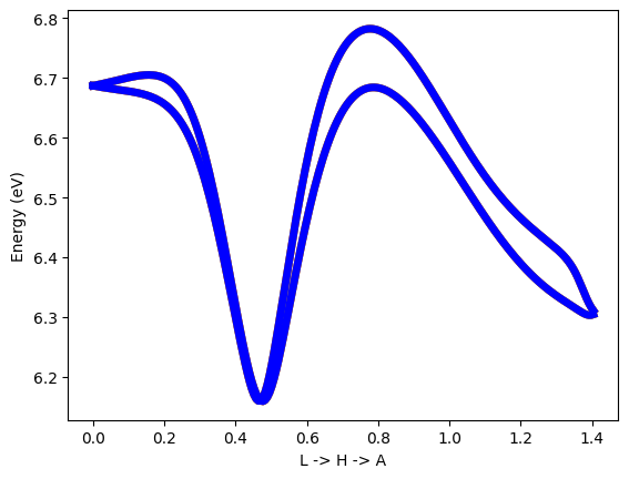
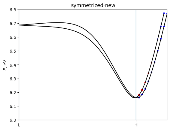
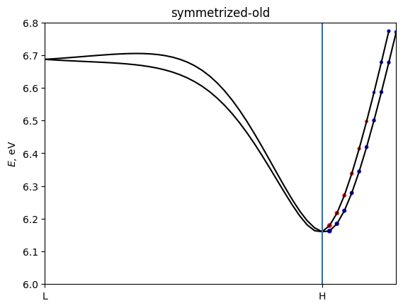
Checking band structures in k-space.
The Brillouin zone of trigonal Te is: 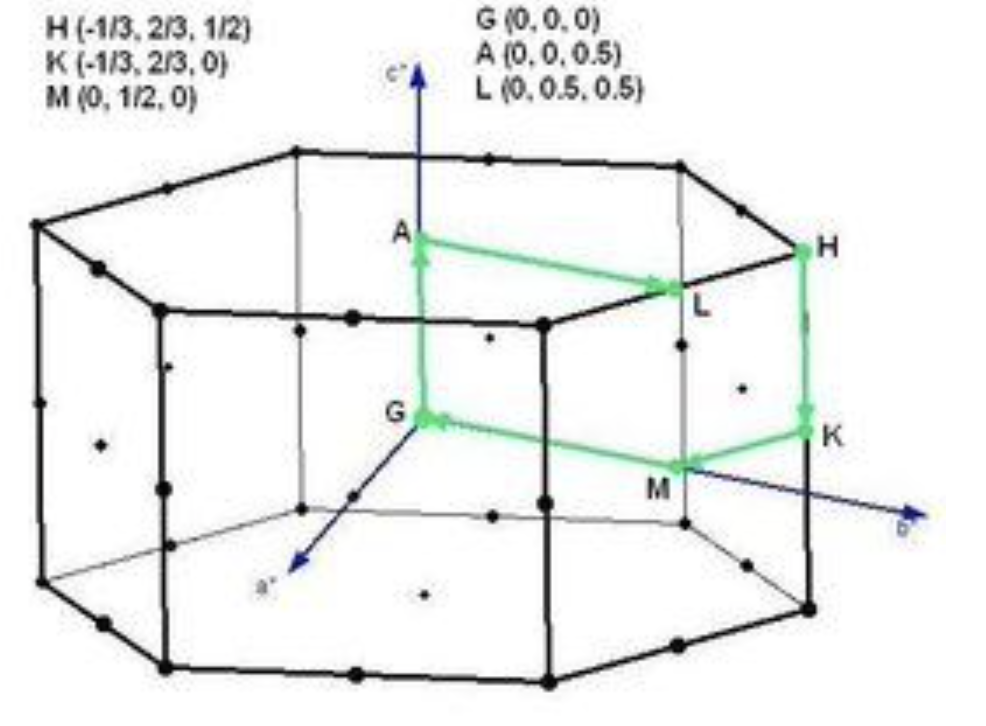 We only consider kz=\(\pi\) plane.
 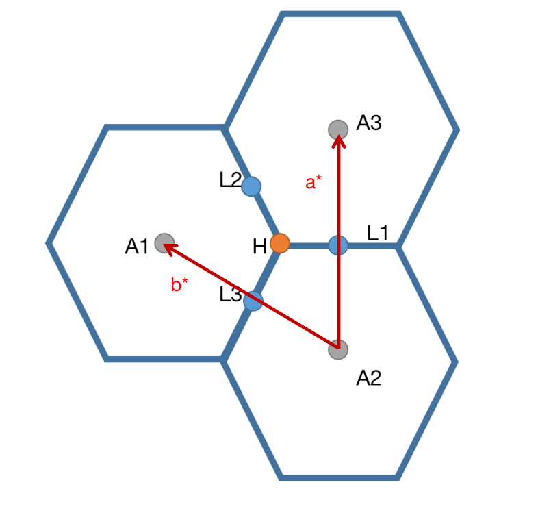 The band structures of the three path:
L1 -> H -> A1
L2 -> H -> A2
L3 -> H -> A3
should be the same because of C3 rotation symmetry.
But the Wannier Hamitonian break the symmetries slightly. So the band structure of the three path may not the same.
After symmetrization they are the same.
[23]:
#generate k-path
path=wberri.Path.from_nodes(system_Te,
    #start and end points of k_path.
    #If two paths are not consencutive, put `None` between them.
    nodes=[[0,0.5,0.5],[1./3,1./3,0.5],[1.,0.,0.5],None,
            [0.5,0.,0.5],[1./3,1./3,0.5],[0.,1.,0.5],None,
            [0.5,0.5,0.5],[1./3,1./3,0.5],[0.,0.,0.5]],
    labels=["L1","H","A1","L3","H","A3","L2","H","A2"],
    #length: proportional to number of kpoints.
    length=1000)


bands_Te = wberri.evaluate_k_path(path = path,  system = system_Te)
bands_Te_sym = wberri.evaluate_k_path(path = path, system = system_Te_sym_new)
Starting run()
Using the follwing calculators :
############################################################

 'tabulate'  :  <wannierberri.calculators.tabulate.TabulatorAll object at 0x787852785430>  :
    TabulatorAll - a pack of all k-resolved calculators (Tabulators)

 Includes the following tabulators :
--------------------------------------------------
 "Energy" : <wannierberri.calculators.tabulate.Energy object at 0x78783be21970> : calculator not described

--------------------------------------------------

############################################################
Calculation along a path - checking calculators for compatibility
tabulate <wannierberri.calculators.tabulate.TabulatorAll object at 0x787852785430>
All calculators are compatible
Symmetrization switched off for Path
Grid is regular
The set of k points is a Path() with 678 points and labels {0: 'L1', 75: 'H', 225: 'A1', 226: 'L3', 301: 'H', 451: 'A3', 452: 'L2', 527: 'H', 677: 'A2'}
generating K_list
Done
Done, sum of weights:678.0

############################################################
Iteration 0 out of 0
processing 678 K points : using  16 processes.
# K-points calculated  Wall time (sec)  Est. remaining (sec)   Est. total (sec)
/home/stepan/github/wannier-berri/wannierberri/grid/path.py:272: UserWarning: symmetry is not used for a tabulation along path
  warnings.warn("symmetry is not used for a tabulation along path")
time for processing    678 K-points on  16 processes:     1.1667 ; per K-point          0.0017 ; proc-sec per K-point          0.0275
time1 =  2.384185791015625e-07
Totally processed 678 K-points
run() finished
Starting run()
Using the follwing calculators :
############################################################

 'tabulate'  :  <wannierberri.calculators.tabulate.TabulatorAll object at 0x78785012d1c0>  :
    TabulatorAll - a pack of all k-resolved calculators (Tabulators)

 Includes the following tabulators :
--------------------------------------------------
 "Energy" : <wannierberri.calculators.tabulate.Energy object at 0x78785012cfe0> : calculator not described

--------------------------------------------------

############################################################
Calculation along a path - checking calculators for compatibility
tabulate <wannierberri.calculators.tabulate.TabulatorAll object at 0x78785012d1c0>
All calculators are compatible
Symmetrization switched off for Path
Grid is regular
The set of k points is a Path() with 678 points and labels {0: 'L1', 75: 'H', 225: 'A1', 226: 'L3', 301: 'H', 451: 'A3', 452: 'L2', 527: 'H', 677: 'A2'}
generating K_list
Done
Done, sum of weights:678.0

############################################################
Iteration 0 out of 0
processing 678 K points : using  16 processes.
# K-points calculated  Wall time (sec)  Est. remaining (sec)   Est. total (sec)
time for processing    678 K-points on  16 processes:     1.1043 ; per K-point          0.0016 ; proc-sec per K-point          0.0261
time1 =  2.384185791015625e-07
Totally processed 678 K-points
run() finished
[24]:
#read energy eigenvalue data of band 18 and 19 from results.
band_Te_01 = bands_Te.get_data(quantity='Energy',iband=(0,1))
band_Te_sym_01 = bands_Te_sym.get_data(quantity='Energy',iband=(0,1))
#read k-path data
band_k=path.getKline()
[27]:
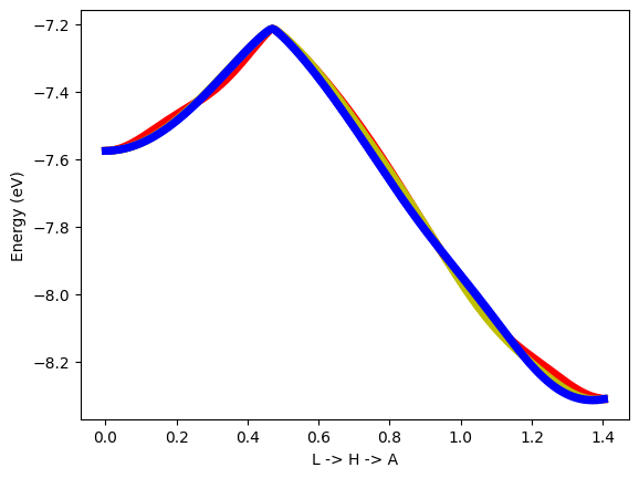
#plot band structure with unsymmetrized system
%matplotlib inline
NK=len(band_k)
colour = ['r','y','b']
NK_one = NK//3
plt.figure()
for i in range(3):
    plt.plot(band_k[0:NK_one],band_Te_01[NK_one*i:NK_one*(i+1)],colour[i],linewidth=1)
plt.ylabel('Energy (eV)')
plt.xlabel('L -> H -> A')
[27]:
Text(0.5, 0, 'L -> H -> A')
[28]:
#plot band structure with symmetrized system
plt.figure()
for i in range(3):
    plt.plot(band_k[0:NK_one],band_Te_sym_01[NK_one*i:NK_one*(i+1)],colour[i],linewidth=1)
plt.ylabel('Energy (eV)')
plt.xlabel('L -> H -> A')
[28]:
Text(0.5, 0, 'L -> H -> A')
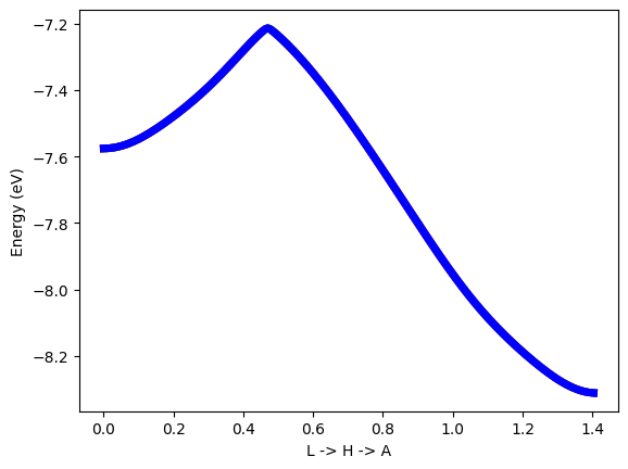
Symmetrization fix the symmetries of Hamiltonian
The Berry curvature is more sensitive to symmetry than energy eigenvalues.
[34]:
# calculate Berry curvature alone a k-path.
path_berry=wberri.Path.from_nodes(system_Te,
                 nodes=[[0,0.5,0.5],[1./3,1./3,0.5],[1./3,1./3,0.]],
                 labels=["L","H","K",],
                 length=500)

quantities = {"Energy":wberri.calculators.tabulate.Energy(),
              "berry":wberri.calculators.tabulate.BerryCurvature(),}

calculators={}
calculators ["tabulate"] = wberri.calculators.TabulatorAll(quantities,ibands=[18,19],mode="path")

berry_Te = wberri.evaluate_k_path(system=system_Te,
        path=path_berry,
        quantities=["berry_curvature"] )

berry_Te_sym = wberri.evaluate_k_path(system=system_Te_sym_new,
        path=path_berry,
        quantities=["berry_curvature"] )

berry_Te_sym_old = wberri.evaluate_k_path(system=system_Te_sym_old,
        path=path_berry,
        quantities=["berry_curvature"] )
Starting run()
Using the follwing calculators :
############################################################

 'tabulate'  :  <wannierberri.calculators.tabulate.TabulatorAll object at 0x78783a9bd970>  :
    TabulatorAll - a pack of all k-resolved calculators (Tabulators)

 Includes the following tabulators :
--------------------------------------------------
 "berry_curvature" : <wannierberri.calculators.tabulate.BerryCurvature object at 0x7879d1162b10> :  Berry curvature :math:`\Omega_a` in units of angstrom^2

 "Energy" : <wannierberri.calculators.tabulate.Energy object at 0x78783a88c7d0> : calculator not described

--------------------------------------------------

############################################################
Calculation along a path - checking calculators for compatibility
tabulate <wannierberri.calculators.tabulate.TabulatorAll object at 0x78783a9bd970>
All calculators are compatible
Symmetrization switched off for Path
Grid is regular
The set of k points is a Path() with 80 points and labels {0: 'L', 37: 'H', 79: 'K'}
generating K_list
Done
Done, sum of weights:80.0

############################################################
Iteration 0 out of 0
processing 80 K points : using  16 processes.
# K-points calculated  Wall time (sec)  Est. remaining (sec)   Est. total (sec)
/home/stepan/github/wannier-berri/wannierberri/grid/path.py:272: UserWarning: symmetry is not used for a tabulation along path
  warnings.warn("symmetry is not used for a tabulation along path")
time for processing     80 K-points on  16 processes:     0.3541 ; per K-point          0.0044 ; proc-sec per K-point          0.0708
time1 =  2.384185791015625e-07
Totally processed 80 K-points
run() finished
Starting run()
Using the follwing calculators :
############################################################

 'tabulate'  :  <wannierberri.calculators.tabulate.TabulatorAll object at 0x78783a92fb90>  :
    TabulatorAll - a pack of all k-resolved calculators (Tabulators)

 Includes the following tabulators :
--------------------------------------------------
 "berry_curvature" : <wannierberri.calculators.tabulate.BerryCurvature object at 0x7879d1162b10> :  Berry curvature :math:`\Omega_a` in units of angstrom^2

 "Energy" : <wannierberri.calculators.tabulate.Energy object at 0x78783bc5f980> : calculator not described

--------------------------------------------------

############################################################
Calculation along a path - checking calculators for compatibility
tabulate <wannierberri.calculators.tabulate.TabulatorAll object at 0x78783a92fb90>
All calculators are compatible
Symmetrization switched off for Path
Grid is regular
The set of k points is a Path() with 80 points and labels {0: 'L', 37: 'H', 79: 'K'}
generating K_list
Done
Done, sum of weights:80.0

############################################################
Iteration 0 out of 0
processing 80 K points : using  16 processes.
# K-points calculated  Wall time (sec)  Est. remaining (sec)   Est. total (sec)
time for processing     80 K-points on  16 processes:     0.8309 ; per K-point          0.0104 ; proc-sec per K-point          0.1662
time1 =  2.384185791015625e-07
Totally processed 80 K-points
run() finished
Starting run()
Using the follwing calculators :
############################################################

 'tabulate'  :  <wannierberri.calculators.tabulate.TabulatorAll object at 0x78783a83b9b0>  :
    TabulatorAll - a pack of all k-resolved calculators (Tabulators)

 Includes the following tabulators :
--------------------------------------------------
 "berry_curvature" : <wannierberri.calculators.tabulate.BerryCurvature object at 0x7879d1162b10> :  Berry curvature :math:`\Omega_a` in units of angstrom^2

 "Energy" : <wannierberri.calculators.tabulate.Energy object at 0x78783b9e9370> : calculator not described

--------------------------------------------------

############################################################
Calculation along a path - checking calculators for compatibility
tabulate <wannierberri.calculators.tabulate.TabulatorAll object at 0x78783a83b9b0>
All calculators are compatible
Symmetrization switched off for Path
Grid is regular
The set of k points is a Path() with 80 points and labels {0: 'L', 37: 'H', 79: 'K'}
generating K_list
Done
Done, sum of weights:80.0

############################################################
Iteration 0 out of 0
processing 80 K points : using  16 processes.
# K-points calculated  Wall time (sec)  Est. remaining (sec)   Est. total (sec)
time for processing     80 K-points on  16 processes:     0.8161 ; per K-point          0.0102 ; proc-sec per K-point          0.1632
time1 =  2.384185791015625e-07
Totally processed 80 K-points
run() finished
[39]:
# use built-in plotting method to plot berry cuvature.
# red means positive, blue means negative.
# size of the dots shows the amplitude of the quantity.
# unsymmetrized:
import matplotlib
# matplotlib.use('TkAgg')


for name, bands in [('unsymmetrized', berry_Te),
                    ('symmetrized-new', berry_Te_sym),
                    ('symmetrized-old', berry_Te_sym_old)]:
    bands.plot_path_fat(path_berry,
              quantity='berry_curvature',
              component='z', # only take z compoment
              Emin=6.0,  Emax=6.8,
              mode="fatband",
              fatfactor=20,  # size of dots.
              close_fig=False,
              )
    plt.title(name)
    plt.show()
    plt.close()
/home/stepan/github/wannier-berri/wannierberri/result/tabresult.py:382: UserWarning: FigureCanvasAgg is non-interactive, and thus cannot be shown
  fig.show()
/home/stepan/github/wannier-berri/wannierberri/result/tabresult.py:382: UserWarning: FigureCanvasAgg is non-interactive, and thus cannot be shown
  fig.show()
/home/stepan/github/wannier-berri/wannierberri/result/tabresult.py:382: UserWarning: FigureCanvasAgg is non-interactive, and thus cannot be shown
  fig.show()
z-component of Berry curvature alone L-H path should be zero because of symmetry. The loss of symmetry has a big impact to Berry curvature of single k-point. It is fixed by symmetrization.
Magnetic system with SOC (bcc Fe)
bcc Fe is a magnetic system with magnetic moment -2.31 \mu_B point to -z direction of cartesian coordinate system of lattice. We need to set parameter ‘magmom’.
[73]:
from irrep.spacegroup import SpaceGroup
from wannierberri.symmetry.sawf import SymmetrizerSAWF
from wannierberri.symmetry.projections import Projection, ProjectionsSet

system_Fe=wberri.System_R.from_tb_dat(tb_file='./Fe_data/Fe_tb.dat',berry=True)
system_Fe_sym_new=wberri.System_R.from_tb_dat(tb_file='./Fe_data/Fe_tb.dat',berry=True)
system_Fe_sym_old=wberri.System_R.from_tb_dat(tb_file='./Fe_data/Fe_tb.dat',berry=True)

spacegroup = SpaceGroup.from_cell(cell=(system_Fe.real_lattice, [[0,0,0]], [1]), magmom=[[0,0,1]], include_TR=True, spinor=True)

proj_sp3d2 = Projection(position_num=[[0,0,0]], orbital="sp3d2", spacegroup=spacegroup)
proj_t2g = Projection(position_num=[[0,0,0]], orbital="t2g", spacegroup=spacegroup)
proj_set = ProjectionsSet([proj_sp3d2, proj_t2g])
# rotate_basis is irrelevant here, because there is only one atom

symmetrizer = SymmetrizerSAWF.from_spacegroup_and_projections(spacegroup=spacegroup, projections=proj_set)
system_Fe_sym_new.symmetrize2(symmetrizer)

system_Fe_sym_old.symmetrize(
             proj = ['Fe:sp3d2;t2g'],
            #  proj = ['Fe:sp3d2','Fe:t2g'],
             atom_name = ['Fe'],
             positions = [[0,0,0]],
             #magmom: magnetic moment of each atoms.
             magmom = [[0.,0.,-2]],
             soc=True,
             )
reading TB file ./Fe_data/Fe_tb.dat ( written on 13May2022 at 01:23:14 )
Real-space lattice:
 [[ 1.4349963  1.4349963  1.4349963]
 [-1.4349963  1.4349963  1.4349963]
 [-1.4349963 -1.4349963  1.4349963]]
Number of wannier functions: 18
Number of R points: 27
Recommended size of FFT grid [5 5 5]
Reading the system from ./Fe_data/Fe_tb.dat finished successfully
num_blocks_left = 2, num_blocks_right = 2
number o R-vectors before symmetrization: 27
number o R-vectors after symmetrization: 27


 ---------- CRYSTAL STRUCTURE ----------


Cell vectors in angstroms:

      Vectors of DFT cell
a0 =  1.4350   1.4350   1.4350
a1 = -1.4350   1.4350   1.4350
a2 = -1.4350  -1.4350   1.4350


 ---------- SPACE GROUP -----------


Space group: I4/mm'm' (# 139.537)
Number of symmetries: 16 (mod. lattice translations)

 ### 1

rotation : |  1   0   0 |
           |  0   1   0 |
           |  0   0   1 |


 gk = [kx, ky, kz]

spinor rot.         : | 1.000+0.000j  0.000+0.000j |
                      | 0.000+0.000j  1.000+0.000j |

translation         :  [   0.0000   0.0000   0.0000 ]

axis: [ 0.040875 -0.315963  0.94789 ] ; angle =  0 , inversion: False, time reversal: False

 ### 2

rotation : | -1   0   0 |
           |  0  -1   0 |
           |  0   0  -1 |


 gk = [-kx, -ky, -kz]

spinor rot.         : | 1.000+0.000j  0.000+0.000j |
                      | 0.000+0.000j  1.000+0.000j |

translation         :  [   0.0000   0.0000   0.0000 ]

axis: [-0.040875 -0.315963  0.94789 ] ; angle =  0 , inversion: True, time reversal: False

 ### 3

rotation : |  0   0   1 |
           |  1   0  -1 |
           |  0   1   1 |


 gk = [kx-ky+kz, kx, ky]

spinor rot.         : | 0.707-0.707j  0.000-0.000j |
                      | 0.000-0.000j  0.707+0.707j |

translation         :  [   0.0000   0.0000   0.0000 ]

axis: [0. 0. 1.] ; angle = 1/2 pi, inversion: False, time reversal: False

 ### 4

rotation : |  0   0  -1 |
           | -1   0   1 |
           |  0  -1  -1 |


 gk = [-kx+ky-kz, -kx, -ky]

spinor rot.         : | 0.707-0.707j  0.000-0.000j |
                      | 0.000-0.000j  0.707+0.707j |

translation         :  [   0.0000   0.0000   0.0000 ]

axis: [0. 0. 1.] ; angle = 1/2 pi, inversion: True, time reversal: False

 ### 5

rotation : |  0   1   1 |
           |  0  -1   0 |
           |  1   1   0 |


 gk = [kz, kx-ky+kz, kx]

spinor rot.         : | 0.000-1.000j -0.000-0.000j |
                      | 0.000-0.000j  0.000+1.000j |

translation         :  [   0.0000   0.0000   0.0000 ]

axis: [0. 0. 1.] ; angle = 1 pi, inversion: False, time reversal: False

 ### 6

rotation : |  0  -1  -1 |
           |  0   1   0 |
           | -1  -1   0 |


 gk = [-kz, -kx+ky-kz, -kx]

spinor rot.         : | 0.000+1.000j -0.000-0.000j |
                      | 0.000-0.000j  0.000-1.000j |

translation         :  [   0.0000   0.0000   0.0000 ]

axis: [ 0.  0. -1.] ; angle = 1 pi, inversion: True, time reversal: False

 ### 7

rotation : |  1   1   0 |
           | -1   0   1 |
           |  1   0   0 |


 gk = [ky, kz, kx-ky+kz]

spinor rot.         : | 0.707+0.707j  0.000+0.000j |
                      |-0.000+0.000j  0.707-0.707j |

translation         :  [   0.0000   0.0000   0.0000 ]

axis: [0. 0. 1.] ; angle = -1/2 pi, inversion: False, time reversal: False

 ### 8

rotation : | -1  -1   0 |
           |  1   0  -1 |
           | -1   0   0 |


 gk = [-ky, -kz, -kx+ky-kz]

spinor rot.         : | 0.707+0.707j  0.000+0.000j |
                      |-0.000+0.000j  0.707-0.707j |

translation         :  [   0.0000   0.0000   0.0000 ]

axis: [0. 0. 1.] ; angle = -1/2 pi, inversion: True, time reversal: False

 ### 9

rotation : |  0  -1  -1 |
           | -1   0   1 |
           |  0   0  -1 |


 gk = [ky, kx, kx-ky+kz]

spinor rot.         : | 0.000+0.000j  0.000-1.000j |
                      | 0.000-1.000j  0.000+0.000j |

translation         :  [   0.0000   0.0000   0.0000 ]

axis: [1. 0. 0.] ; angle = 1 pi, inversion: False, time reversal: True

 ### 10

rotation : |  0   1   1 |
           |  1   0  -1 |
           |  0   0   1 |


 gk = [-ky, -kx, -kx+ky-kz]

spinor rot.         : | 0.000+0.000j  0.000-1.000j |
                      | 0.000-1.000j  0.000+0.000j |

translation         :  [   0.0000   0.0000   0.0000 ]

axis: [1. 0. 0.] ; angle = 1 pi, inversion: True, time reversal: True

 ### 11

rotation : | -1  -1   0 |
           |  0   1   0 |
           |  0  -1  -1 |


 gk = [kx, kx-ky+kz, kz]

spinor rot.         : |-0.000+0.000j  0.707-0.707j |
                      |-0.707-0.707j  0.000+0.000j |

translation         :  [   0.0000   0.0000   0.0000 ]

axis: [ 0.707107 -0.707107  0.      ] ; angle = 1 pi, inversion: False, time reversal: True

 ### 12

rotation : |  1   1   0 |
           |  0  -1   0 |
           |  0   1   1 |


 gk = [-kx, -kx+ky-kz, -kz]

spinor rot.         : |-0.000+0.000j -0.707+0.707j |
                      | 0.707+0.707j  0.000+0.000j |

translation         :  [   0.0000   0.0000   0.0000 ]

axis: [-0.707107  0.707107 -0.      ] ; angle = 1 pi, inversion: True, time reversal: True

 ### 13

rotation : | -1   0   0 |
           |  1   0  -1 |
           | -1  -1   0 |


 gk = [kx-ky+kz, kz, ky]

spinor rot.         : | 0.000-0.000j -1.000+0.000j |
                      | 1.000+0.000j  0.000+0.000j |

translation         :  [   0.0000   0.0000   0.0000 ]

axis: [-0.  1.  0.] ; angle = 1 pi, inversion: False, time reversal: True

 ### 14

rotation : |  1   0   0 |
           | -1   0   1 |
           |  1   1   0 |


 gk = [-kx+ky-kz, -kz, -ky]

spinor rot.         : | 0.000+0.000j -1.000+0.000j |
                      | 1.000+0.000j  0.000+0.000j |

translation         :  [   0.0000   0.0000   0.0000 ]

axis: [0. 1. 0.] ; angle = 1 pi, inversion: True, time reversal: True

 ### 15

rotation : |  0   0  -1 |
           |  0  -1   0 |
           | -1   0   0 |


 gk = [kz, ky, kx]

spinor rot.         : |-0.000+0.000j -0.707-0.707j |
                      | 0.707-0.707j  0.000+0.000j |

translation         :  [   0.0000   0.0000   0.0000 ]

axis: [0.707107 0.707107 0.      ] ; angle = 1 pi, inversion: False, time reversal: True

 ### 16

rotation : |  0   0   1 |
           |  0   1   0 |
           |  1   0   0 |


 gk = [-kz, -ky, -kx]

spinor rot.         : |-0.000+0.000j  0.707+0.707j |
                      |-0.707+0.707j  0.000+0.000j |

translation         :  [   0.0000   0.0000   0.0000 ]

axis: [-0.707107 -0.707107 -0.      ] ; angle = 1 pi, inversion: True, time reversal: True
pos_list: [[0]]
proj: Projection 0, 0, 0:['sp3d2;t2g'] with 18 Wannier functions (9 per spin x2 spins)
 on 1 points (18 per site)
orbital = sp3d2;t2g, num wann per site = 18
new_wann_indices: [0, 1, 2, 3, 4, 5, 6, 7, 8, 9, 10, 11, 12, 13, 14, 15, 16, 17]
/home/stepan/github/wannier-berri/wannierberri/system/system_R.py:370: UserWarning: for effeciency of symmetrization, it is recommended to give orbitals separately, not combined by a ';' sign.But you need to do it consistently in wannier90
  warnings.warn("for effeciency of symmetrization, it is recommended to give orbitals separately, not combined by a ';' sign."
num_blocks_left = 1, num_blocks_right = 1
number o R-vectors before symmetrization: 27
number o R-vectors after symmetrization: 27
[73]:
<wannierberri.symmetry.sawf.SymmetrizerSAWF at 0x78783bc4ade0>
Important explanations: 1. The projection card in wannier90.win of bcc Fe is 'Fe':sp3d2;dxz,dyz,dxy. But in the symmetrization, orbitals must project to complete sets of coordinates after symmetry opration. So we must label orbitals which shares the same complete sets of coordinates. eg: sp3d2, dxz,dyz,dxy -> sp3d2, t2g and sp,px,py -> sp,p2 2. We print out all the symmetry operators in the space group. But magnetic moments break some of them. Afte line Symmetrizing start. You
can find details about which operator belong to the magnetic group.
bcc Fe have inversion symmetry, so the Berry curvature dipole should be zero. Ref: https://journals.aps.org/prl/pdf/10.1103/PhysRevLett.115.216806
[75]:
system_Fe_sym = system_Fe_sym_new
#calculate berry curvature dipole
Efermi_Fe = np.linspace(15.5,16,301)
NK = 24

grid = wberri.Grid(system_Fe,NK=NK,NKFFT=6)

results_Fe = {}

for name, system in [('unsymmetrized', system_Fe),
                     ('symmetrized-new', system_Fe_sym_new),
                     ('symmetrized-old', system_Fe_sym_old)]:

    results_Fe[name] = wberri.run(system=system,
            grid=grid,
            calculators = {"BerryDipole":wberri.calculators.static.BerryDipole_FermiSea(Efermi=Efermi_Fe,tetra=False)},
            adpt_num_iter=0,
            fout_name=f'Fe-{name}',
            use_irred_kpt=False,
            symmetrize=False,
            )
Starting run()
Using the follwing calculators :
############################################################

 'BerryDipole'  :  <wannierberri.calculators.static.BerryDipole_FermiSea object at 0x7878201a3ef0>  : Berry curvature dipole (dimensionless)

        | With Fermi sea integral. Eq(29) in `Ref <https://www.nature.com/articles/s41524-021-00498-5>`__
        | Output: :math:`D_{\beta\delta} = \int [dk] \partial_\beta \Omega_\delta f`
############################################################
Calculation on  grid - checking calculators for compatibility
BerryDipole <wannierberri.calculators.static.BerryDipole_FermiSea object at 0x7878201a3ef0>
All calculators are compatible
Grid is regular
The set of k points is a Grid() with NKdiv=[4 4 4], NKFFT=[6 6 6], NKtot=[24 24 24]
generating K_list
Done in 0.00021791458129882812 s
K_list contains 64 Irreducible points(100.0%) out of initial 4x4x4=64 grid
Done, sum of weights:1.0

############################################################
Iteration 0 out of 0
processing 64 K points : using  16 processes.
# K-points calculated  Wall time (sec)  Est. remaining (sec)   Est. total (sec)
time for processing     64 K-points on  16 processes:     5.8703 ; per K-point          0.0917 ; proc-sec per K-point          1.4676
time1 =  2.384185791015625e-07
Totally processed 64 K-points
run() finished
Starting run()
Using the follwing calculators :
############################################################

 'BerryDipole'  :  <wannierberri.calculators.static.BerryDipole_FermiSea object at 0x787820276450>  : Berry curvature dipole (dimensionless)

        | With Fermi sea integral. Eq(29) in `Ref <https://www.nature.com/articles/s41524-021-00498-5>`__
        | Output: :math:`D_{\beta\delta} = \int [dk] \partial_\beta \Omega_\delta f`
############################################################
Calculation on  grid - checking calculators for compatibility
BerryDipole <wannierberri.calculators.static.BerryDipole_FermiSea object at 0x787820276450>
All calculators are compatible
Grid is regular
The set of k points is a Grid() with NKdiv=[4 4 4], NKFFT=[6 6 6], NKtot=[24 24 24]
generating K_list
Done in 0.0002129077911376953 s
K_list contains 64 Irreducible points(100.0%) out of initial 4x4x4=64 grid
Done, sum of weights:1.0

############################################################
Iteration 0 out of 0
processing 64 K points : using  16 processes.
# K-points calculated  Wall time (sec)  Est. remaining (sec)   Est. total (sec)
                  48              5.1                   1.7                   6.7
time for processing     64 K-points on  16 processes:     5.9322 ; per K-point          0.0927 ; proc-sec per K-point          1.4830
time1 =  2.384185791015625e-07
Totally processed 64 K-points
run() finished
Starting run()
Using the follwing calculators :
############################################################

 'BerryDipole'  :  <wannierberri.calculators.static.BerryDipole_FermiSea object at 0x78783a94e960>  : Berry curvature dipole (dimensionless)

        | With Fermi sea integral. Eq(29) in `Ref <https://www.nature.com/articles/s41524-021-00498-5>`__
        | Output: :math:`D_{\beta\delta} = \int [dk] \partial_\beta \Omega_\delta f`
############################################################
Calculation on  grid - checking calculators for compatibility
BerryDipole <wannierberri.calculators.static.BerryDipole_FermiSea object at 0x78783a94e960>
All calculators are compatible
Grid is regular
The set of k points is a Grid() with NKdiv=[4 4 4], NKFFT=[6 6 6], NKtot=[24 24 24]
generating K_list
Done in 0.00018477439880371094 s
K_list contains 64 Irreducible points(100.0%) out of initial 4x4x4=64 grid
Done, sum of weights:1.0

############################################################
Iteration 0 out of 0
processing 64 K points : using  16 processes.
# K-points calculated  Wall time (sec)  Est. remaining (sec)   Est. total (sec)
time for processing     64 K-points on  16 processes:     5.9973 ; per K-point          0.0937 ; proc-sec per K-point          1.4993
time1 =  2.384185791015625e-07
Totally processed 64 K-points
run() finished
[81]:
#read data

Fe_BCD = results_Fe['unsymmetrized'].results["BerryDipole"].data
Fe_sym_BCD = results_Fe['symmetrized-new'].results["BerryDipole"].data
Fe_sym_old_BCD = results_Fe['symmetrized-old'].results["BerryDipole"].data
plt.plot(Efermi_Fe,Fe_BCD[:,2,2],'r',label="Unsymmetrized")
plt.plot(Efermi_Fe,Fe_sym_BCD[:,2,2],'b--',label="Symmetrized")
plt.plot(Efermi_Fe,Fe_sym_old_BCD[:,2,2],'g:',label="Symmetrized-old")
plt.legend()
plt.xlabel('Energy (eV)')
plt.ylabel('Berry curvature dipole')
[81]:
Text(0, 0.5, 'Berry curvature dipole')
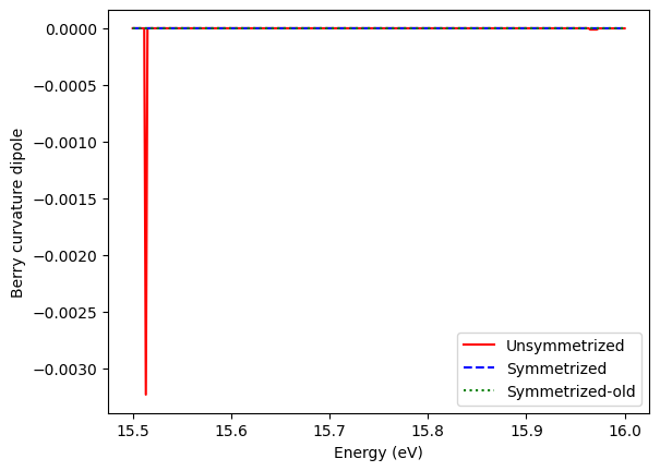
Symmetrized system gives us better results with low-density k-grid. But it still looks like not perfect zero. At some energy where have band intersections, we can see some little peaks come from digital error. There are very large Berry curvature and it’s divergent around band intersections. They may enlarge digital errors.